List of Figures

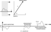	Figure 1: Schematic response of two-way Doppler tracking to a GW. The Doppler exhibits three pulses having amplitudes and relative locations which depend on the GW arrival direction, the two-way light time, and the wave’s strain amplitude and polarization state. The sum of the three pulses is zero, so the pulses overlap and partially cancel when the characteristic time of the GW pulse is comparable to or larger than the light time between the earth and spacecraft.
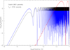	Figure 2: Polarization-averaged power response of the Doppler system to a gravitational wave signal as a function of Fourier frequency. Earth-spacecraft geometry for Cassini’s gravity wave observations in 2000 – 2001 has been used. Blue: response from the direction of Virgo ( $μ ≃$ 0.104). Black: response to randomly polarized sources distributed isotropically on the celestial sphere. Red: response from the direction of the galactic center ( $μ ≃$ 0.9932). Note that in the case of waves from the Galactic center, the three-pulse response function ([52] and Eq. (1 *)) for the Cassini geometry is dominated by two pulses separated by only about 0.00034 T₂ $≃$ 20 s. This gives rise to the strong low-frequency suppression and the approximate sin² modulation for the Cassini GWE1 geometry and GWs from the galactic center. BepubtkUpdateB2Corrected sign error for $μ$ to galactic center in Figure 2.
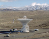	Figure 3: DSS 25, a 34-m beam-waveguide antenna, shown here in the stowed position. DSS 25 is one antenna in the NASA/JPL Goldstone Deep Space Communications Complex near Barstow, CA, U.S.A. It has special instrumentation (Ka-band up- and downlink and advanced tropospheric calibration capability) which enable particularly good quality Doppler observations. BepubtkUpdateB3Replaced Figure 3 with a different photograph.
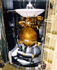	Figure 4: The Cassini spacecraft during pre-launch testing. Reference [37] gives a popular discussion of the Cassini mission, the spacecraft, and its instrumentation (photograph courtesy NASA/JPL-Caltech).
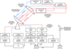	Figure 5: Conceptual sketch of signal flow for two-way Cassini observations, with emphasis on showing which links are affected by specific noise sources. For example, spacecraft buffeting and the frequency and timing subsystem (FTS) are common to all Doppler links. The Ka-band translator (KaT) affects only the Ka2 downlink, while the conventional transponder (KEX) affects both the X-downlink and the Ka1 downlink, etc.
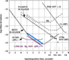	Figure 6: Allan deviation (square root of Allan variance [23]) as a function of integration time for several frequency and timing technologies in the Cassini-era. The technology used in precision Doppler observations for GW searches with Cassini has $σy$ (1000 s) less than 10^–15. (Figure courtesy of Lute Maleki; see also references [10, 11, 22].)
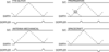	Figure 7: Schematic transfer functions of noises to the two-way Doppler link, adapted from [46, 125]. For each type of disturbance a separate diagram (space vertically, time horizontally) is shown. Radio waves propagate continuously up to and down from the spacecraft; some of these are represented as the dashed lines to illustrate the indicated Doppler frequency perturbations. For example, a momentary glitch in the FTS affects the frequency reference for both the receiver and the transmitter. This shows up as an immediate effect in the received Doppler (difference between the transmitted and received frequency). Because the glitch also affects the transmitted frequency, it shows up again – but with the opposite sense – in the Doppler after a two-way light time. These various noise responses contrast with the three-pulse GW response, shown in Figure 1; these differences are exploited in the signal processing.
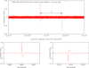	Figure 8: Time series of Cassini two-way Ka-band frequency residuals from a DSS 25 track on 2001 DOY 350. The data are sampled at 0.2 s after being detected with a time constant $≃$ 1 s. At this time resolution, the visual appearance of the time series is dominated by high-frequency noise. Superimposed on this noise are two systematic glitches which were traced to an intermittently-faulty distribution amplifier in the signal chain providing frequency references to the transmitter and receiver. The distribution amplifier fault acts like an FTS glitch and, in the two-way Doppler, appears twice in the time series anticorrelated at the two-way light time (Figure 7). The glitches in the figure are paired with the indicated two-way light time separation T₂ $≃$ 5737.7 s. The lower panels show blowups of the pair; the glitch waveforms are unresolved (shapes set by the impulse response of the software phase detector) but clearly show the characteristic FTS anticorrelation.
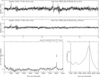	Figure 9: Doppler time series for DSS 25 Cassini track on 2003 DOY 324. Upper panel: time series of the two-way X-band, showing two discrete events at about 10:20 and 10:40 ground received time, echoed about a two way light time, T₂, later. Middle panel: time series of X-(880/3344) Ka1, which isolates the downlink plasma (and cancels nondispersive noises and signals: FTS, troposphere, antenna mechanical noise, and GWs). This shows that the events observed in the upper panel are due to plasma scintillation. Lower panel: acf of the two-way Doppler time series. The arrow marks the two-way light time. The lower right panel is a blow-up of the acf near the two-way light time (indicated by the vertical line). The acf peaks at lags slightly smaller than T₂ $≃$ 8021.5 s, indicating that the features observed in the upper panels are caused by near-earth plasma.AepubtkUpdateA2Modified figure to discuss the blowup of the acf.
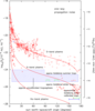	Figure 10: Summary of propagation and antenna mechanical noises as functions of sun-earth-spacecraft angle (updated from [22], reproduced by permission of the American Geophysical Union; see also [131, 21, 65, 9, 10, 11, 122, 121]). Left axis: spectral density of fractional frequency fluctuations at f = 0.001 Hz. Right axis: fractional frequency fluctuation (Allan deviation $σy$ ) at $τ$ = 1000 s. S-band $≃$ 2.3 GHz; X-band $≃$ 8.4 GHz; Ka-band $≃$ 32 GHz. Red curves are for plasma scintillation at the indicated radio frequencies (circles are S-band, more precisely: S-(3/11)X differential frequency fluctuations, data from Viking [131, 21]); crosses are X-band (more precisely X-(880/3344) Ka1 differential frequency fluctuations, from Cassini [122, 11, 19, 29, 121]). Blue region shows typical uncalibrated tropospheric scintillation levels at a moderate-altitude dry site such as Goldstone, CA, or the National Radio Astronomy Observatory’s Very Large Array [20, 75, 76]. Green arrows show upper (for antennas in the DSN “high efficiency” sub-network, operated under operational but benign conditions) and lower (for DSS 25, near solar opposition) limits to antenna mechanical noise [9, 19, 22]. AepubtkUpdateA4Updated Figure 10. BepubtkUpdateB5Replaced Figure 10 with updated version containing new data.
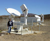	Figure 11: Two water-vapor-radiometer-based Advanced Media Calibration units located near DSS 25, shown here in November 2001. These are used to calibrate tropospheric phase scintillation for the Cassini Gravitational Wave Experiment and other Cassini precision Doppler tracking observations. (Mark Gatti, project manager for the Cassini Radio Science ground system upgrades, is in the foreground.)
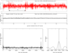	Figure 12: Doppler time series for DSS 25 Cassini track on 2001 DOY 330, showing an antenna mechanical noise event. Upper panel: time series of the two-way Ka-band, with approximately 10 s time resolution. The middle panel shows the time series of X-(880/3344) Ka1, i.e., essentially the X-band plasma on the downlink, indicating the low level of plasma noise on this day. The AMC data similarly show low tropospheric noise. The event at about 07:30 is echoed about a two-way light time later, and may be due to gusting wind on this day (another candidate pair is at about 09:45 and a two-way light time later). The lower left panel shows the autocorrelation of the two-way Ka-band data, peaking at T₂ $≃$ 5717.9 s. The lower right panel is a blow-up of the acf near the lag of a two-way light time (indicated by the vertical line).
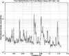	Figure 13: Spectrum of Cassini radial velocity fluctuations, observed in a 40-hour cruise test during 2001 DOY 152-153 [129], reproduced here with permission. The Allan deviation associated with this spacecraft buffeting noise [52, 46] is 2.3 × 10^–16 at an integration time of 1000 s.
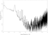	Figure 14: Power spectrum of the two-way fractional frequency fluctuations (calibrated for plasma and troposphere) for 2001 – 2002 Cassini solar opposition observations (adapted from [19]). The spectrum has been smoothed from the intrinsic resolution of the observations to a bandwidth of $≃$ 3 $μ$ Hz to reduce estimation error. Representative 95% confidence limits are indicated.
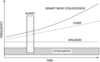	Figure 15: Schematic diagram of signals in a frequency-time space. Sinusoids are “on” for all time and have horizontal tracks, linear chirps are straight lines with non-zero slope, bursts are time-localized, etc. These localizations in frequency-time suggest different detection approaches for different classes of signal. This space can be tiled in many ways. Particular tilings can have special merit for particular waveforms, e.g., if a candidate signal projects preferentially onto a small fraction of a particular mathematical basis while the noise does not.
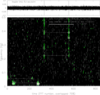	Figure 16: Frequency-time representation of Cassini two-way Ka-band data on 2001 DOY 350. Upper panel: time series of two-way Doppler data with $≃$ 1 s time constant, sampled at 0.2 s/sample. At this resolution the visual impression of the plot is set by relatively high frequency noise. Lower right panel: low frequency resolution power spectrum of the full data set shown in upper panel. Lower left panel: normalized dynamic spectrum of the data in the upper panel. This was constructed by forming sequential spectra of short ( $≃$ 102 s) unwindowed segments of the data. Each data segment is 75% overlapped with its neighbors. The heavy white line indicates the two-way light time at the beginning of the data set. The plotted quantity is power at a given point in (frequency-time) divided by a local estimate of the average power at that (frequency, time) point, a nondimensional measure of the contrast of the Fourier power at that point relative to an estimated background. The color code runs from black (low values) through green (higher values) to red (very high values). Points with this estimated contrast ratio > 10 are marked with white circles. If two high-contrast features are at the same frequency and separated by a two-way light time, they are connected with a thin white line. The FTS glitch shown also in Figure 8 is clearly evident in both the time series and in T₂-separated bands of high-contrast Fourier power in the lower plot. Additional features paired at T₂ in the earlier, lower-frequency part of the data are also detected in the normalized dynamic spectrum.
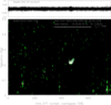	Figure 17: As for Figure 16, but for the Cassini two-way Ka-band track on 2003 DOY 008. The strong features in the dynamic spectrum at about (08:50, 0.22 Hz) have peak local contrast > 100 (and are even marginally visible in the time series in the upper panel).
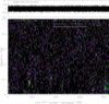	Figure 18: As for Figure 17, but for the Cassini two-way X-band track on 2003 DOY 008. Note the absence of high-contrast features near (08:50 UT, 0.22 Hz).
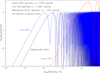	Figure 19: Power response of the Doppler system to a gravitational-wave signal, as a function of Fourier frequency, for signals from the direction of the galactic center. Blue: Juno 2016 opportunity. Black: BepiColombo 2019+ opportunity. Red: Cassini 2001 geometry.
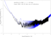	Figure 20: Sensitivity of the Cassini 2001 – 2002 gravitational wave observations, expressed as the equivalent sinusoidal strain sensitivity required to produce SNR = 1 for a randomly polarized isotropic background as a function of Fourier frequency. This reflects both the levels, spectral shapes, and transfer functions of the instrumental noises (see Section 4) and the GW transfer function (see Section 3). Black curve: sensitivity computed using smoothed version of observed noise spectrum; blue curve: sensitivity computed from pre-observation predicted noise spectrum [111].
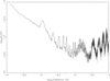	Figure 21: Characteristic all-sky strain sensitivity for a burst wave having a bandwidth comparable to center frequency for the Cassini 2001 – 2002 data set [19]. This is the crudest measure of sky-averaged burst sensitivity: the square root of the product of the Doppler spectrum and the Fourier frequency, divided by the sky-averaged GW response (see Section 6.4).
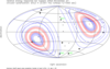	Figure 22: Contours of constant matched filter output for a wave having $h+ (t) = sin(2πt ⋅ 0.001 Hz)exp (− t∕1000 s)H (t)$ and $h ×(t)$ its Hilbert transform, adapted from [64]. Cassini November 2003 geometry is assumed (the red dot is the right ascension and declination of Cassini). Black dots are the positions of members of the Local Group of galaxies. “GC” marks the location of the galactic center. Contour levels are at 1/10 of the maximum, with red contours at 0.9 to 0.5 of the maximum signal output and blue contours at 0.4 to 0.1. Doppler response is zero in the direction of Cassini (and its anti-direction).
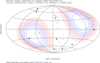	Figure 23: As in Figure 22 but for a wave with $h+ (t) = sin(2πt ⋅ 0.0001 Hz )exp(− t∕10000 s)H (t)$ and $h×(t)$ its Hilbert transform. This model waveform is long compared with T₂.
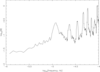	Figure 24: Upper limits to the energy density of GWs in bandwidth equal to center frequency, relative to closure energy density. This assumes an isotropic GW background, H₀ = 75 km s^–1 Mpc^–1, and is computed from the Cassini 2001 – 2002 data [19].
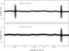	Figure 25: Time series of DSS 14 two-way (upper panel) and DSS 25 three way (lower panel) Doppler during the 2007 March 15 antenna mechancial noise test. At about 04:30 UT the subreflector at DSS 14 was deliberately articulated to produce large antenna mechanical noise variation. The effect in the two-way Doppler is seen immediately and at a two-way light time (T₂ = 8341.6 s) later (see Figure 7). The receive-only three-way station is unaffected at 04:30 UT (it is receiving a signal transmitted a two-way light time earlier) but observes the effect of the deliberate subreflcetor motion a two-way light time later (lower panel). (The three impulsive glitches in the two-way time series are unrelated to this mechanical noise test.) Figure adapted from [15].AepubtkUpdateA7Added Figure 25.
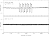	Figure 26: Blowup of DSS 14 two-way Doppler time series (upper panel) near the deliberate subreflector articulation. The lower panel shows the data combination E(t), which cancels the antenna mechanical noise in the two-way time series leaving the antenna mechanical noise of the three-way station (DSS 25) and other secondary noises. Figure adapted from [15].AepubtkUpdateA8Added Figure 26.

	Abstract
1	Introduction
2	Notation, Acronyms, and Conventions
3	Gravitational Wave Signal Response
4	Apparatus and Principal Noise Sources
	4.1	Frequency standard noise
	4.2	Plasma scintillation noise
	4.3	Tropospheric scintillation noise
	4.4	Antenna mechanical noise
	4.5	Ground electronics noise
	4.6	Spacecraft transponder noise
	4.7	Thermal noise in the ground and spacecraft receivers
	4.8	Spacecraft unmodeled motion
	4.9	Numerical noise in orbit removal
	4.10	Aggregate spectrum
	4.11	Summary of noise levels and transfer functions
5	Signal Processing
	5.1	Noise spectrum estimation
	5.2	Sinusoidal and quasiperiodic waves
	5.3	Bursts
	5.4	Stochastic background
	5.5	Classification of data intervals based on transfer functions
	5.6	Frequency-time representations
	5.7	Qualifying/disqualifying candidates
	5.8	Other comments
6	Detector Performance
	6.1	Observations to date
	6.2	Near-future observations
	6.3	Sensitivity to periodic and quasi-periodic waves
	6.4	Burst waves
	6.5	Sensitivity to a stochastic background
7	Improving Doppler Tracking Sensitivity
8	The LISA Low-Frequency Detector
9	Concluding Comments
	Acknowledgements
	References
	Footnotes
	Updates
	Figures
	Tables