3 Gravitational Wave Signal Response
The theory of spacecraft Doppler tracking as a GW detector was developed by Estabrook and Wahlquist [52*]. Briefly, consider the earth and a spacecraft as separated test masses, at rest with respect to one another and separated by distance L = cT2 / 2, where T2 is the two-way light time (light time from the earth to the spacecraft and back). A ground station continuously transmits a nearly monochromatic microwave signal (center frequency ) to the spacecraft. This signal is coherently
transponded by the distant spacecraft and sent back to the earth. The ground station compares the
frequency of the signal which it is transmitting with the frequency of the signal it is receiving. The
two-way fractional frequency fluctuation is
) to the spacecraft. This signal is coherently
transponded by the distant spacecraft and sent back to the earth. The ground station compares the
frequency of the signal which it is transmitting with the frequency of the signal it is receiving. The
two-way fractional frequency fluctuation is ![y2(t) = [ν(t − T2) − ν(t)]∕ν0](article35x.gif) , where
, where  is the
frequency of the actual transmitted signal. In this way the Doppler tracking system measures the
relative dimensionless velocity of the earth and spacecraft:
is the
frequency of the actual transmitted signal. In this way the Doppler tracking system measures the
relative dimensionless velocity of the earth and spacecraft:  . In an idealized
system (no noise, no systematic effects, no gravitational radiation), this time series would be
zero.
. In an idealized
system (no noise, no systematic effects, no gravitational radiation), this time series would be
zero.
A GW incident on this system causes perturbations in the Doppler frequency time series. The
gravitational-wave response  of a two-way Doppler system excited by a transverse, traceless plane
gravitational wave [84] having unit wavevector
of a two-way Doppler system excited by a transverse, traceless plane
gravitational wave [84] having unit wavevector  is [52*]

 =
=  ,
,  is a unit vector from the earth to the spacecraft,
  ,
and
,
and  is the first order metric perturbation at the earth. (Here
  is distinguished from the
  used to analyze the LISA detector [16*, 51*, 119, 120]:
  .) The GW amplitude at
the earth is
.) The GW amplitude at
the earth is ![h (t) = [h+(t)e+ + h×(t)e×]](article49x.gif) , where the 3-tensors
, where the 3-tensors  and
and  are transverse
to
are transverse
to  and, with respect to an orthonormal
  propagation frame, have components
(If general relativity and a transverse traceless perturbation are not assumed, the amplitude of the
three-pulse response for a general tensor metric perturbation is given in [57].)
propagation frame, have components
(If general relativity and a transverse traceless perturbation are not assumed, the amplitude of the
three-pulse response for a general tensor metric perturbation is given in [57].)
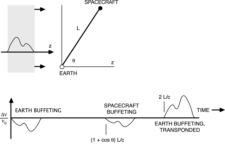
The Doppler responds to a projection of the time-dependent wave metric, in general producing a
“three-pulse” response to a pulse of incident gravitational radiation: one event due to buffeting of the earth
by the GW, one event due to buffeting of the spacecraft by the GW, and a third event in which the original
earth buffeting is transponded a two-way light time later. The amplitudes and locations of the pulses
depend on the arrival direction of the GW with respect to the earth-spacecraft line, the two-way light time,
and the wave’s polarization state. From Eq. (1*) the sum of the three pulses is zero. Since the detector
response depends both on the spacecraft-earth-GW geometry (T2,  ) and the wave properties (Fourier
frequency content, polarization state) its distinctive three-pulse signature plays an important role in
distinguishing candidate signals from competing noises. Figure 1* shows this three pulse response in
schematic form.
) and the wave properties (Fourier
frequency content, polarization state) its distinctive three-pulse signature plays an important role in
distinguishing candidate signals from competing noises. Figure 1* shows this three pulse response in
schematic form.
In the special case of the long-wavelength limit (LWL, where the Fourier frequencies of the GW signal
are  1/T2), the gravitational wave can be expanded in terms of spatial derivatives. Equation (1*) then
gives the LWL response for two-way Doppler tracking:
1/T2), the gravitational wave can be expanded in terms of spatial derivatives. Equation (1*) then
gives the LWL response for two-way Doppler tracking:

 T2, the full three pulse character
[Eq. (1*)] is expressed in the Doppler time series. Figure 2* shows the spectral response of a
Doppler tracking system to sinusoidal GW signals from two specific directions and the average
response from sources distributed isotropically on the celestial sphere. Because Figure 2* plots
the transfer function to the spectral power, the dependence at low-frequency is
T2, the full three pulse character
[Eq. (1*)] is expressed in the Doppler time series. Figure 2* shows the spectral response of a
Doppler tracking system to sinusoidal GW signals from two specific directions and the average
response from sources distributed isotropically on the celestial sphere. Because Figure 2* plots
the transfer function to the spectral power, the dependence at low-frequency is  f2. The
algorithm used to average over GW polarization states in Figure 2* is described in [18*, 16*]. A
related discussion (how to infer GW amplitudes, h – or limits to h – from measurements of
y2 when the signal direction and polarization state are unknown) is in [18*]. The LWL of the
three-pulse GW response has been used to analyze the GW response of ground-based Michelson
gravitational wave interferometers [47]. The three-pulse response can also be constructed using the
formalism of time-delay interferometry, the method LISA will use to cancel laser phase noise in an
unequal-arm spaceborne GW detector (see Section 8). The formalism has also been applied
to analysis of other spaceborne detector geometries, for example the candidate linear array,
SyZyGy [49].
f2. The
algorithm used to average over GW polarization states in Figure 2* is described in [18*, 16*]. A
related discussion (how to infer GW amplitudes, h – or limits to h – from measurements of
y2 when the signal direction and polarization state are unknown) is in [18*]. The LWL of the
three-pulse GW response has been used to analyze the GW response of ground-based Michelson
gravitational wave interferometers [47]. The three-pulse response can also be constructed using the
formalism of time-delay interferometry, the method LISA will use to cancel laser phase noise in an
unequal-arm spaceborne GW detector (see Section 8). The formalism has also been applied
to analysis of other spaceborne detector geometries, for example the candidate linear array,
SyZyGy [49].
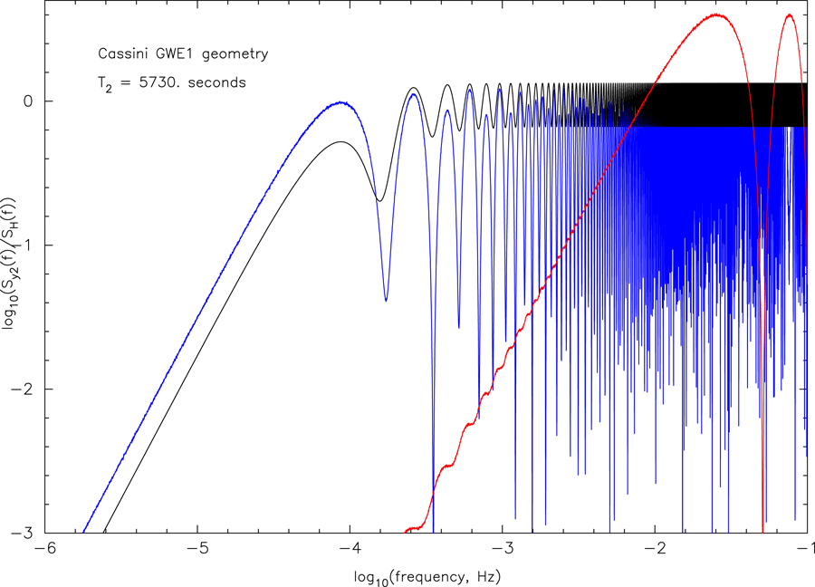
 0.104). Black:
response to randomly polarized sources distributed isotropically on the celestial sphere. Red: response
from the direction of the galactic center (
0.104). Black:
response to randomly polarized sources distributed isotropically on the celestial sphere. Red: response
from the direction of the galactic center ( 0.9932). Note that in the case of waves from the
Galactic center, the three-pulse response function ([52*] and Eq. (1*)) for the Cassini geometry is
dominated by two pulses separated by only about 0.00034 T2
0.9932). Note that in the case of waves from the
Galactic center, the three-pulse response function ([52*] and Eq. (1*)) for the Cassini geometry is
dominated by two pulses separated by only about 0.00034 T2  20 s. This gives rise to the strong
low-frequency suppression and the approximate sin2 modulation for the Cassini GWE1 geometry
and GWs from the galactic center. Update*
20 s. This gives rise to the strong
low-frequency suppression and the approximate sin2 modulation for the Cassini GWE1 geometry
and GWs from the galactic center. Update*In a practical GW observation spanning 20 – 40 days, the earth-spacecraft distance and the orientation of the earth-spacecraft vector on the celestial sphere change (typically slowly) with time. This modifies the idealized GW response (it is not strictly time-shift invariant) and has practical consequences in searches for long-lived signals (see Section 5.7).
To summarize the Doppler signal response:
- GW signals are observed in the Doppler tracking time series through the three pulse response [Eq. (1*)].
- The response depends on the two-way light time T2, the cosine of the angle between the GW
wavevector and unit vector from the earth to the spacecraft, and GW properties (Fourier
content and polarization state) [Eq. (1*)] and the expression for
 ).
).
- The GW response is not in general time-shift invariant if T2 or
 change during the time of
observation.
change during the time of
observation.
- The GW response is a high-pass filter: In the long-wavelength limit (frequencies
 1/T/sub2), the response is attenuated due to pulse overlap and cancellation (see
Figure 2*).
1/T/sub2), the response is attenuated due to pulse overlap and cancellation (see
Figure 2*).
 |
 |
 |