7 Experimental Aspects of TDI
It is clear that the suppression of the laser phase fluctuations by more than nine orders of magnitude with the use of TDI is a very challenging experimental task. It requires developing and building subsystems capable of unprecedented accuracy and precision levels, and test their end-to-end performance in a laboratory environment that naturally precludes the availability of km delay lines! In what follows
we will address some aspects related to the experimental implementation of TDI, and derive the
performance specifications for the subsystems involved. We will not address, however, any of
the experimental aspects related to the verification of TDI in a laboratory environment. For
that, we refer the interested reader to de Vine et al. [8*, 32*], Spero et al. [48*], and Mitryk et
al. [33*].
km delay lines! In what follows
we will address some aspects related to the experimental implementation of TDI, and derive the
performance specifications for the subsystems involved. We will not address, however, any of
the experimental aspects related to the verification of TDI in a laboratory environment. For
that, we refer the interested reader to de Vine et al. [8*, 32*], Spero et al. [48*], and Mitryk et
al. [33*].
From simple physical grounds, it is easy to see that a successful implementation of TDI requires:
- accurate knowledge of the time shifts,
 , to be applied to the heterodyne
measurements
, to be applied to the heterodyne
measurements  ;
;
- accurate synchronization among the three clocks onboard the three spacecraft as these are used for time-stamping the recorded heterodyne phase measurements;
- sampling time stability (i.e., clock stability) for successfully suppressing the laser noise to the desired level;
- an accurate reconstruction algorithm of the phase measurements corresponding to the required time delays as these in general will not be equal to integer multiples of the sampling time;
- a phase meter capable of a very large dynamic range in order to suppress the laser noise to the required level while still preserving the phase fluctuations induced by a gravitational-wave signal in the TDI combinations.
In the following subsections, we will quantitatively address the issues listed above, and provide the reader with a related list of references where more details can be found.
7.1 Time-delays accuracies
The TDI combinations described in the previous sections (whether of the first- or second-generation) rely on
the assumption of knowing the time-delays with infinite accuracy to exactly cancel the laser noise. Since the
six delays will in fact be known only within the accuracies  , the cancellation of the
laser frequency fluctuations in, for instance, the combinations (
, the cancellation of the
laser frequency fluctuations in, for instance, the combinations ( ) will no longer be exact. In
order to estimate the magnitude of the laser fluctuations remaining in these data sets, let us
define
) will no longer be exact. In
order to estimate the magnitude of the laser fluctuations remaining in these data sets, let us
define  to be the estimated time-delays. They are related to the true delays
 , and the accuracies
 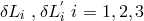 through the following expressions

 as constants equal to 16.7 light-seconds. We will also assume to know with infinite
accuracies and precisions all the remaining physical quantities (listed at the beginning of Section 7) that
are needed to successfully synthesize the TDI generators.
as constants equal to 16.7 light-seconds. We will also assume to know with infinite
accuracies and precisions all the remaining physical quantities (listed at the beginning of Section 7) that
are needed to successfully synthesize the TDI generators.
If we now substitute Eq. (98*) into the expression for the TDI combination  , for instance, (Eq. (43*))
and expand it to first order in
, for instance, (Eq. (43*))
and expand it to first order in  , it is easy to derive the following approximate expression for
  ,
which now will show a non-zero contribution from the laser noises
,
which now will show a non-zero contribution from the laser noises
![αˆ(t) ≃ α (t) + [ ˙ϕ2,12 − ˙ϕ3,13] δL1 + [ϕ ˙3,2 − ˙ϕ1,123] δL2 + [ϕ˙1,123 − ˙ϕ2,3] δL3 , (99 )](article905x.gif)
 denotes time derivative. Time-delay interferometry can be considered effective if the
magnitude of the remaining fluctuations from the lasers are much smaller than the fluctuations due to the
remaining (proof mass and optical path) noises entering
denotes time derivative. Time-delay interferometry can be considered effective if the
magnitude of the remaining fluctuations from the lasers are much smaller than the fluctuations due to the
remaining (proof mass and optical path) noises entering  . This requirement implies a limit in the
accuracies of the measured delays.
. This requirement implies a limit in the
accuracies of the measured delays.
Let us assume the laser phase fluctuations to be uncorrelated to each other, their one-sided power
spectral densities to be equal, the three armlengths to differ by a few percent, and the three armlength
accuracies also to be equal. By requiring the magnitude of the remaining laser noises to be smaller than the
secondary noise sources, it is straightforward to derive, from Eq. (99*) and the expressions for the noise
spectrum of the  TDI combination given in [15*], the following constraint on the common armlength
accuracy
TDI combination given in [15*], the following constraint on the common armlength
accuracy 
![∘ ------2----------------2------------------------------------- |δL | ≪ √--1--- [8-sin--(3-πfL-) +-16-sin-(πf-L-)]-S-proof mass(f) +-S-optical path(f)-, (100 ) α 32πf S ϕ(f)](article910x.gif)
 and
and  . Here
  ,
,  ,
,  are the
one-sided power spectral densities of the relative frequency fluctuations of a stabilized laser, a single proof
mass, and a single-link optical path respectively. If we take them to be equal to the following functions of
the Fourier frequency
are the
one-sided power spectral densities of the relative frequency fluctuations of a stabilized laser, a single proof
mass, and a single-link optical path respectively. If we take them to be equal to the following functions of
the Fourier frequency  [53, 15]
(where
[53, 15]
(where 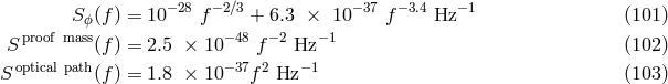
 is in Hz), we find that the right-hand side of the inequality given by Eq. (100*) reaches its
minimum of about 30 meters at the Fourier frequency
is in Hz), we find that the right-hand side of the inequality given by Eq. (100*) reaches its
minimum of about 30 meters at the Fourier frequency  , over the assumed
(
, over the assumed
( ) Hz LISA band. This implies that, if the armlength knowledge
  can be made much
smaller than 30 meters, the magnitude of the residual laser noise affecting the
can be made much
smaller than 30 meters, the magnitude of the residual laser noise affecting the  combination can be
regarded as negligible over the entire frequency band. This reflects the fact that the armlength accuracy is a
decreasing function of the frequency. For instance, at
combination can be
regarded as negligible over the entire frequency band. This reflects the fact that the armlength accuracy is a
decreasing function of the frequency. For instance, at  the armlength accuracy goes up by almost
an order of magnitude to about 155 meters.
the armlength accuracy goes up by almost
an order of magnitude to about 155 meters.
A perturbation analysis similar to the one described above can be performed for  , resulting into the
following inequality for the required delay accuracy,
, resulting into the
following inequality for the required delay accuracy, 

 , while at
  the armlength accuracy goes up to
154 meters.
the armlength accuracy goes up to
154 meters.
Armlength accuracies at the centimeters level have already been demonstrated in the laboratory [16*, 50*, 64*, 26*], making us confident that the required level of time-delays accuracy will be available.
In relation to the accuracies derived above, it is interesting to calculate the time scales during which the armlengths will change by an amount equal to the accuracies themselves. This identifies the minimum time required before updating the armlength values in the TDI combinations.
It has been calculated by Folkner et al. [21*] that the relative longitudinal speeds between the three pairs of spacecraft, during approximately the first year of the LISA mission, can be written in the following approximate form
where we have denoted with
 the three possible spacecraft pairs,
  is a constant
velocity, and
is a constant
velocity, and  is the period for the pair
  . In reference [21*] it has also been shown that the
LISA trajectory can be selected in such a way that two of the three arms’ rates of change are
essentially equal during the first year of the mission. Following reference [21], we will assume
. In reference [21*] it has also been shown that the
LISA trajectory can be selected in such a way that two of the three arms’ rates of change are
essentially equal during the first year of the mission. Following reference [21], we will assume
 , with
  ,
,  ,
,  months, and
 year. From Eq. (105*) it is easy to derive the variation of each armlength, for example
 , as a function of the time
  and the time scale
  during which it takes place
Equation (106*) implies that a variation in armlength
during which it takes place
Equation (106*) implies that a variation in armlength 
 can take place during different time
scales, depending on when during the mission this change takes place. For instance, if
can take place during different time
scales, depending on when during the mission this change takes place. For instance, if  we find
that the armlength
we find
that the armlength  changes by more than its accuracy (
 ) after a time
  . If
however
. If
however  , the armlength will change by the same amount after only
  instead. As this
value is less than the one-way-light-time, one might argue that the measured time-delay will not represent
well enough the delay that needs to be applied in the TDI combinations at that particular
time.
instead. As this
value is less than the one-way-light-time, one might argue that the measured time-delay will not represent
well enough the delay that needs to be applied in the TDI combinations at that particular
time.
One way to address this problem is to treat the delays in the TDI combinations as parameters to be determined by a non-linear least-squares procedure, in which the minimum of the minimizer is achieved at the correct delays since that the laser noise will exactly cancel there in the TDI combinations. Such a technique, which was named time-delay interferometric ranging (TDIR) [60], requires a starting point in the time-delays space in order to implement the minimization, and it will work quite effectively jointly with the ranging data available onboard.
7.2 Clocks synchronization
The effectiveness of the TDI data combinations requires the clocks onboard the three spacecraft to be synchronized. In what follows we will identify the minimum level of off-synchronization among the clocks that can be tolerated. In order to proceed with our analysis we will treat one of the three clocks (say the clock onboard spacecraft 1) as the master clock defining the time for LISA, while the other two to be synchronized to it.
The relativistic (Sagnac) time-delay effect due to the fact that the LISA trajectory is a combination of two rotations, each with a period of one year, will have to be accounted for in the synchronization procedure and, as has already been discussed earlier, will be accounted for within the second-generation formulation of TDI.
Here, for simplicity, we will analyze an idealized non-rotating constellation in order to get a sense of the
required level of clocks synchronization. Let us denote by  ,
,  , the time accuracies (time-offsets) for
the clocks onboard spacecraft 2 and 3 respectively. If
, the time accuracies (time-offsets) for
the clocks onboard spacecraft 2 and 3 respectively. If  is the time onboard spacecraft 1, then what is
believed to be time
is the time onboard spacecraft 1, then what is
believed to be time  onboard spacecraft 2 and 3 is actually equal to the following times
 , for instance, and expand it to first
order in
, for instance, and expand it to first
order in  , it is easy to derive the following approximate expression for
  , which shows the
following non-zero contribution from the laser noises
By requiring again the magnitude of the remaining fluctuations from the lasers to be smaller than the
fluctuations due to the other (secondary) noise sources affecting
, which shows the
following non-zero contribution from the laser noises
By requiring again the magnitude of the remaining fluctuations from the lasers to be smaller than the
fluctuations due to the other (secondary) noise sources affecting ![ˆζ(t) ≃ ζ(t) + [ ˙ϕ − ˙ϕ + ϕ˙ − ϕ˙ ] δt + [ ˙ϕ − ϕ˙ + ϕ˙ − ϕ˙ ] δt . (109 ) 1,23 3,12 2,13 2,13 2 2,13 1,23 3,12 3,12 3](article958x.gif)
 , it is possible to derive an upper
limit for the accuracies of the synchronization of the clocks. If we assume again the three laser phase
fluctuations to be uncorrelated to each other, their one-sided power spectral densities to be equal, the three
armlengths to differ by a few percent, and the two time-offsets’ magnitudes to be equal, by
requiring the magnitude of the remaining laser noises to be smaller than the secondary noise
sources it is easy to derive the following constraint on the time synchronization accuracy
, it is possible to derive an upper
limit for the accuracies of the synchronization of the clocks. If we assume again the three laser phase
fluctuations to be uncorrelated to each other, their one-sided power spectral densities to be equal, the three
armlengths to differ by a few percent, and the two time-offsets’ magnitudes to be equal, by
requiring the magnitude of the remaining laser noises to be smaller than the secondary noise
sources it is easy to derive the following constraint on the time synchronization accuracy  with
with 
 ,
,  ,
,  again as given in Eqs. (101* – 103*).
We find that the right-hand side of the inequality given by Eq. (110*) reaches its minimum of
about 47 nanoseconds at the Fourier frequency  . This means that clocks
synchronized at a level of accuracy significantly better than 47 nanoseconds will result into a
residual laser noise that is much smaller than the secondary noise sources entering into the
. This means that clocks
synchronized at a level of accuracy significantly better than 47 nanoseconds will result into a
residual laser noise that is much smaller than the secondary noise sources entering into the  combination.
An analysis similar to the one described above can be performed for the remaining generators
( ). For them we find that the corresponding inequality for the accuracy in the synchronization of
the clocks is now equal to
). For them we find that the corresponding inequality for the accuracy in the synchronization of
the clocks is now equal to
![∘ -------------------------------------------------------------- 2 2 proof mass optical path |δtα | ≤ --1- [4-sin-(3πf-L)-+-8-sin-(πfL-)] S--------(f)-+-3-S---------(f-), (111 ) 2πf 4 S ϕ(f)](article968x.gif)
 and
and  . The function on the right-hand side of Eq. (111*) has a
minimum equal to 88 nanoseconds at the Fourier frequency
. The function on the right-hand side of Eq. (111*) has a
minimum equal to 88 nanoseconds at the Fourier frequency 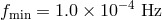 . As for the armlength
accuracies, also the timing accuracy requirements become less stringent at higher frequencies. At
. As for the armlength
accuracies, also the timing accuracy requirements become less stringent at higher frequencies. At
 , for instance, the timing accuracy for
  and
and  go up to 446 and 500 ns
respectively.
go up to 446 and 500 ns
respectively.
As a final note, a required clock synchronizations of about 40 ns derived in this section translates into a ranging accuracy of 12 meters, which has been experimentally shown to be easily achievable [16, 50, 64, 26].
7.3 Clocks timing jitter
The sampling times of all the measurements needed for synthesizing the TDI combinations will not be
constant, due to the intrinsic timing jitters of the onboard measuring system. Among all the subsystems
involved in the data measuring process, the onboard clock is expected to be the dominant source of
time jitter in the sampled data. Presently existing space qualified clocks can achieve an Allan
standard deviation of about  for integration times from 1 to 10 000 seconds. This timing
stability translates into a time jitter of about
for integration times from 1 to 10 000 seconds. This timing
stability translates into a time jitter of about  seconds over a period of 1 second. A
perturbation analysis including the three sampling time jitters due to the three clocks shows that
any laser phase fluctuations remaining in the four TDI generators will also be proportional to
the sampling time jitters. Since the latter are approximately four orders of magnitude smaller
than the armlength and clocks synchronization accuracies derived earlier, we conclude that the
magnitude of laser noise residual into the TDI combinations due to the sampling time jitters is
negligible.
seconds over a period of 1 second. A
perturbation analysis including the three sampling time jitters due to the three clocks shows that
any laser phase fluctuations remaining in the four TDI generators will also be proportional to
the sampling time jitters. Since the latter are approximately four orders of magnitude smaller
than the armlength and clocks synchronization accuracies derived earlier, we conclude that the
magnitude of laser noise residual into the TDI combinations due to the sampling time jitters is
negligible.
7.4 Sampling reconstruction algorithm
The derivations of the time-delays and clocks synchronization accuracies highlighted earlier presumed the availability of the phase measurement samples at the required time-delays. Since this condition will not be true in general, as the time-delays used by the TDI combinations will not be equal to integer-multiples of the sampling time, with a sampling rate of, let us say, 10 Hz, the time delays could be off their correct values by a tenth of a second, way more than the 10 nanoseconds time-delays and clocks synchronization accuracies estimated above.
Earlier suggestions [27*] for addressing this problem envisioned sampling the data at very-high rates (perhaps of the order of hundreds of MHz), so reducing the additional error to the estimated time-delays to a few nanoseconds. Although in principle such a solution would allow us to suppress the residual laser noise to the required level, it would create an insurmountable problem for transmitting the science data to the ground due to the limited space-to-ground data rates.
An alternate scheme for obtaining the phase measurement points needed by TDI [59*] envisioned sampling the phase measurements at the required delayed times. This scheme naturally requires knowledge of the time-delays and synchronization of the clocks at the required accuracy levels during data acquisition. Although such a procedure could be feasible in principle, it would still leave open the possibility of irreversible corruption of the TDI combinations in the eventuality of performance degradation in the ranging and clock synchronization procedures.
Given that the data will need to be sampled at a rate of 10 Hz, an alternative options is to implement an interpolation scheme for reconstructing the required data points from the sampled measurements. An analysis [59*] based on the implementation of the truncated Shannon [47] formula, however, showed that several months of data were required in order to reconstruct the phase samples at the estimated time-delays with a sufficiently high accuracy. This conclusion implied that several months (at the beginning and end) of the entire data records measured by LISA would be of no use, resulting into a significant mission science degradation.
Although the truncated Shannon formula was proved to be impracticable [59*] for reconstructing phase samples at the required time-delays, it was then recognized that [46*] a more efficient and accurate interpolation technique [31] could be adopted. In what follows, we provide a brief account of this data processing technique, which is known as “fractional-delay filtering” (FDF).
In order to understand how FDF works, let’s write the truncated Shannon formula for the
delayed sample,  , which we want to construct by filtering the sampled data
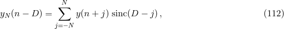
 , and
, and  is an integer at which the Shannon formula has been
truncated to. As pointed out in [46*], although the truncated Shannon formula is optimal in the
least-squares sense, the sinc-function that appears in it is far from being ideal in reconstructing the transfer
function
is an integer at which the Shannon formula has been
truncated to. As pointed out in [46*], although the truncated Shannon formula is optimal in the
least-squares sense, the sinc-function that appears in it is far from being ideal in reconstructing the transfer
function  , where
  is the sampling frequency. In fact, over the LISA observational band the
sinc-function displays significant ringing, which can only be suppressed by taking
is the sampling frequency. In fact, over the LISA observational band the
sinc-function displays significant ringing, which can only be suppressed by taking  very large (as the
error,
very large (as the
error,  , decays slowly as
  ). It was estimated that, in order to achieve an
  , an
, an  is needed.
If, however, we give up on the requirement of minimizing the error in the least-squares sense
and replace it with a mini-max criterion error applied to the absolute value of the difference
between the ideal transfer function (i.e.,  ) and a modified sinc-function, we will be able
to achieve a rapid convergence while suppressing the ringing effects associated with the sinc
function.
) and a modified sinc-function, we will be able
to achieve a rapid convergence while suppressing the ringing effects associated with the sinc
function.
One way to achieve this result is to modify the Shannon formula by multiplying the sinc-function by a
window-function,  , in the following way

 smoothly decays to zero at
  . In [46*] several windows were tested, and the resulting
values of
. In [46*] several windows were tested, and the resulting
values of  needed to accurately reconstruct the desired delayed samples were estimated, both on
theoretical and numerically grounds. It was found that, with windows belonging to the family of Lagrange
polynomials [46] a delayed sample could be reconstructed by using
needed to accurately reconstruct the desired delayed samples were estimated, both on
theoretical and numerically grounds. It was found that, with windows belonging to the family of Lagrange
polynomials [46] a delayed sample could be reconstructed by using  samples while achieving a
mini-max error
samples while achieving a
mini-max error  between the ideal transfer function
  , and the kernel of the modified
truncated Shannon formula.
, and the kernel of the modified
truncated Shannon formula.
7.5 Data digitization and bit-accuracy requirement
It has been shown [59] that the maximum of the ratio between the amplitudes of the laser and the
secondary phase fluctuations occurs at the lower end of the LISA bandwidth (i.e., 0.1 mHz) and it is
equal to about  . This corresponds to the minimum dynamic range for the phasemeters to
correctly measure the laser fluctuations and the weaker (gravitational-wave) signals simultaneously.
An additional safety factor of
. This corresponds to the minimum dynamic range for the phasemeters to
correctly measure the laser fluctuations and the weaker (gravitational-wave) signals simultaneously.
An additional safety factor of  should be sufficient to avoid saturation if the noises are
well described by Gaussian statistics. In terms of requirements on the digital signal processing
subsystem, this dynamic range implies that approximately 36 bits are needed when combining
the signals in TDI, only to bridge the gap between laser frequency noise and the other noises
and gravitational-wave signals. More bits might be necessary to provide enough information
to efficiently filter the data when extracting weak gravitational-wave signals embedded into
noise.
should be sufficient to avoid saturation if the noises are
well described by Gaussian statistics. In terms of requirements on the digital signal processing
subsystem, this dynamic range implies that approximately 36 bits are needed when combining
the signals in TDI, only to bridge the gap between laser frequency noise and the other noises
and gravitational-wave signals. More bits might be necessary to provide enough information
to efficiently filter the data when extracting weak gravitational-wave signals embedded into
noise.
The phasemeters will be the onboard instrument that will perform the phase measurements containing the gravitational signals. They will also need to simultaneously measure the time-delays to be applied to the TDI combinations via ranging tones over-imposed on the laser beams exchanged by the spacecraft. And they will need to have the capability of simultaneously measure additional side-band tones that are required for the calibration of the onboard Ultra-Stable Oscillator used in the down-conversion of heterodyned carrier signal [57, 27].
Work toward the realization of a phasemeter capable of meeting these very stringent performance and operational requirements has aggressively been performed both in the United States and in Europe [43, 23, 22, 6, 63], and we refer the reader interested in the technical details associated with the development studies of such device to the above references and those therein.
 |
 |
 |
Living Rev. Relativity, 17 (2014), 6, doi:10.12942/lrr-2014-6, URL (accessed <date>): http://www.livingreviews.org/lrr-2014-6.
 This work is licensed under a Creative Commons License.
© The author(s), except where otherwise noted.
This work is licensed under a Creative Commons License.
© The author(s), except where otherwise noted.