4 Algebraic Approach for Canceling Laser and Optical Bench Noises
In ground-based detectors the arms are chosen to be of equal length so that the laser light experiences identical delay in each arm of the interferometer. This arrangement precisely cancels the laser frequency/phase noise at the photodetector. The required sensitivity of the instrument can thus only be achieved by near exact cancellation of the laser frequency noise. However, in LISA it is impossible to achieve equal distances between spacecraft, and the laser noise cannot be canceled in this way. It is possible to combine the recorded data linearly with suitable time-delays corresponding to the three arm lengths of the giant triangular interferometer so that the laser phase noise is canceled. Here we present a systematic method based on modules over polynomial rings which guarantees all the data combinations that cancel both the laser phase and the optical bench motion noises. We first consider the simpler case, where we ignore the optical-bench motion noise and consider only the
laser phase noise. We do this because the algebra is somewhat simpler and the method is easy to apply. The
simplification amounts to physically considering each spacecraft rigidly carrying the assembly of lasers,
beam-splitters, and photodetectors. The two lasers on each spacecraft could be considered to be locked, so
effectively there would be only one laser on each spacecraft. This mathematically amounts to setting
 and
and  . The scheme we describe here for laser phase noise can be extended in a
straight-forward way to include optical bench motion noise, which we address in the last part of this
section.
. The scheme we describe here for laser phase noise can be extended in a
straight-forward way to include optical bench motion noise, which we address in the last part of this
section.
The data combinations, when only the laser phase noise is considered, consist of the six suitably delayed
data streams (inter-spacecraft), the delays being integer multiples of the light travel times between
spacecraft, which can be conveniently expressed in terms of polynomials in the three delay operators  ,
,
 ,
,  . The laser noise cancellation condition puts three constraints on the six polynomials of the delay
operators corresponding to the six data streams. The problem, therefore, consists of finding six-tuples of
polynomials which satisfy the laser noise cancellation constraints. These polynomial tuples form a
module2
called the module of syzygies. There exist standard methods for obtaining the module, by which we mean
methods for obtaining the generators of the module so that the linear combinations of the generators
generate the entire module. The procedure first consists of obtaining a Gröbner basis for the ideal
generated by the coefficients appearing in the constraints. This ideal is in the polynomial ring in the
variables
. The laser noise cancellation condition puts three constraints on the six polynomials of the delay
operators corresponding to the six data streams. The problem, therefore, consists of finding six-tuples of
polynomials which satisfy the laser noise cancellation constraints. These polynomial tuples form a
module2
called the module of syzygies. There exist standard methods for obtaining the module, by which we mean
methods for obtaining the generators of the module so that the linear combinations of the generators
generate the entire module. The procedure first consists of obtaining a Gröbner basis for the ideal
generated by the coefficients appearing in the constraints. This ideal is in the polynomial ring in the
variables  ,
,  ,
,  over the domain of rational numbers (or integers if one gets rid of the
denominators). To obtain the Gröbner basis for the ideal, one may use the Buchberger algorithm or use
an application such as Mathematica [65]. From the Gröbner basis there is a standard way
to obtain a generating set for the required module. This procedure has been described in the
literature [3*, 29*]. We thus obtain seven generators for the module. However, the method does not
guarantee a minimal set and we find that a generating set of 4 polynomial six-tuples suffice to
generate the required module. Alternatively, we can obtain generating sets by using the software
Macaulay 2.
over the domain of rational numbers (or integers if one gets rid of the
denominators). To obtain the Gröbner basis for the ideal, one may use the Buchberger algorithm or use
an application such as Mathematica [65]. From the Gröbner basis there is a standard way
to obtain a generating set for the required module. This procedure has been described in the
literature [3*, 29*]. We thus obtain seven generators for the module. However, the method does not
guarantee a minimal set and we find that a generating set of 4 polynomial six-tuples suffice to
generate the required module. Alternatively, we can obtain generating sets by using the software
Macaulay 2.
The importance of obtaining more data combinations is evident: They provide the necessary redundancy – different data combinations produce different transfer functions for GWs and the system noises so specific data combinations could be optimal for given astrophysical source parameters in the context of maximizing SNR, detection probability, improving parameter estimates, etc.
4.1 Cancellation of laser phase noise
We now only have six data streams  and
and  , where
  . These can be regarded as 3
component vectors
. These can be regarded as 3
component vectors  and
and  , respectively. The six data streams with terms containing only the laser
frequency noise are
, respectively. The six data streams with terms containing only the laser
frequency noise are
Note that we have intentionally excluded from the data additional phase fluctuations due to the GW signal, and noises such as the optical-path noise, proof-mass noise, etc. Since our immediate goal is to cancel the laser frequency noise we have only kept the relevant terms. Combining the streams for canceling the laser frequency noise will introduce transfer functions for the other noises and the GW signal. This is important and will be discussed subsequently in the article.
The goal of the analysis is to add suitably delayed beams together so that the laser frequency noise terms
add up to zero. This amounts to seeking data combinations that cancel the laser frequency noise. In the
notation/formalism that we have invoked, the delay is obtained by applying the operators  to the
beams
to the
beams  and
and  . A delay of
  is represented by the operator
  acting
on the data, where
acting
on the data, where  ,
,  , and
, and  are integers. In general, a polynomial in
  , which is a
polynomial in three variables, applied to, say,
, which is a
polynomial in three variables, applied to, say,  combines the same data stream
  with different
time-delays of the form
with different
time-delays of the form  . This notation conveniently rephrases the problem.
One must find six polynomials say
. This notation conveniently rephrases the problem.
One must find six polynomials say  ,
,  ,
,  , such that
It is useful to express Eq. (16*) in matrix form. This allows us to obtain a matrix operator equation
whose solutions are  and
and  , where
  and
and  are written as column vectors. We can similarly
express
are written as column vectors. We can similarly
express  ,
,  ,
,  as column vectors
  ,
,  ,
,  , respectively. In matrix form Eq. (16*) becomes

 is a
is a  matrix given by
The exponent ‘
matrix given by
The exponent ‘
 ’ represents the transpose of the matrix. Eq. (17*) becomes
where we have taken care to put
’ represents the transpose of the matrix. Eq. (17*) becomes
where we have taken care to put 
 on the right-hand side of the operators. Since the above equation must
be satisfied for an arbitrary vector
on the right-hand side of the operators. Since the above equation must
be satisfied for an arbitrary vector  , we obtain a matrix equation for the polynomials
  :
Note that since the
:
Note that since the 
 commute, the order in writing these operators is unimportant. In mathematical
terms, the polynomials form a commutative ring.
commute, the order in writing these operators is unimportant. In mathematical
terms, the polynomials form a commutative ring.
4.2 Cancellation of laser phase noise in the unequal-arm interferometer
The use of commutative algebra is very conveniently illustrated with the help of the simpler example of the unequal-arm interferometer. Here there are only two arms instead of three as we have for LISA, and the mathematics is much simpler and so it easy to see both physically and mathematically how commutative algebra can be applied to this problem of laser phase noise cancellation. The procedure is well known for the unequal-arm interferometer, but here we will describe the same method but in terms of the delay operators that we have introduced.
Let  denote the laser phase noise entering the laser cavity as shown in Figure 5*. Consider this
light
denote the laser phase noise entering the laser cavity as shown in Figure 5*. Consider this
light  making a round trip around arm 1 whose length we take to be
  . If we interfere this phase
with the incoming light we get the phase
. If we interfere this phase
with the incoming light we get the phase  , where

 , where
Clearly, if
, where
Clearly, if 
 , then the difference in phase
  is not zero and the laser phase noise does
not cancel out. However, if one further delays the phases
is not zero and the laser phase noise does
not cancel out. However, if one further delays the phases  and
and  and constructs the following
combination,
then the laser phase noise does cancel out. We have already encountered this combination at the end of
Section 2. It was first proposed by Tinto and Armstrong in [53*].
and constructs the following
combination,
then the laser phase noise does cancel out. We have already encountered this combination at the end of
Section 2. It was first proposed by Tinto and Armstrong in [53*].
![X (t) = [ϕ2(t − 2L1 ) − ϕ2(t)] − [ϕ1 (t − 2L2 ) − ϕ1(t)], (24 )](article279x.gif)
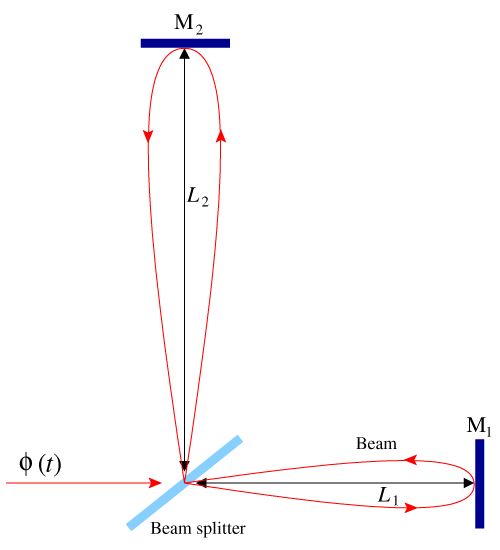
 in
in  which is first sent around arm 1 followed
by arm 2. The second beam (not shown) is first sent around arm 2 and then through arm 1. The
difference in these two beams constitutes
which is first sent around arm 1 followed
by arm 2. The second beam (not shown) is first sent around arm 2 and then through arm 1. The
difference in these two beams constitutes  .
.The cancellation of laser frequency noise becomes obvious from the operator algebra in the following way. In the operator notation,
From this one immediately sees that just the commutativity of the operators has been used to cancel the laser phase noise. The basic idea was to compute the lowest common multiple (L.C.M.) of the polynomials![2 2 X (t) = (𝒟 1 − 1)ϕ2 (t) − (𝒟2 − 1) ϕ1(t) = [(𝒟21 − 1)(𝒟22 − 1) − (𝒟22 − 1)(𝒟21 − 1 )]ϕ (t) = 0. (25 )](article284x.gif)
 and
and  (in this case the L.C.M. is just the product, because the polynomials are relatively
prime) and use this fact to construct
(in this case the L.C.M. is just the product, because the polynomials are relatively
prime) and use this fact to construct  in which the laser phase noise is canceled. The operation is
shown physically in Figure 5*.
in which the laser phase noise is canceled. The operation is
shown physically in Figure 5*.
The notions of commutativity of polynomials, L.C.M., etc. belong to the field of commutative algebra.
In fact we will be using the notion of a Gröbner basis which is in a sense the generalization of the notion of
the greatest common divisor (gcd). Since LISA has three spacecraft and six inter-spacecraft beams, the
problem of the unequal-arm interferometer only gets technically more complex; in principle the problem is
the same as in this simpler case. Thus, the simple operations which were performed here to obtain a laser
noise free combination  are not sufficient and more sophisticated methods need to be
adopted from the field of commutative algebra. We address this problem in the forthcoming
text.
are not sufficient and more sophisticated methods need to be
adopted from the field of commutative algebra. We address this problem in the forthcoming
text.
4.3 The module of syzygies
Equation (21*) has non-trivial solutions. Several solutions have been exhibited in [2*, 15*]. We
merely mention these solutions here; in the forthcoming text we will discuss them in detail.
The solution  is given by
  . The solution
  is described by
 and
and  . The solutions
  and
and  are obtained from
  by
cyclically permuting the indices of
by
cyclically permuting the indices of  ,
,  , and
, and  . These solutions are important, because
they consist of polynomials with lowest possible degrees and thus are simple. Other solutions
containing higher degree polynomials can be generated conveniently from these solutions. Since
the system of equations is linear, linear combinations of these solutions are also solutions to
Eq. (21*).
. These solutions are important, because
they consist of polynomials with lowest possible degrees and thus are simple. Other solutions
containing higher degree polynomials can be generated conveniently from these solutions. Since
the system of equations is linear, linear combinations of these solutions are also solutions to
Eq. (21*).
However, it is important to realize that we do not have a vector space here. Three independent
constraints on a six-tuple do not produce a space which is necessarily generated by three basis elements.
This conclusion would follow if the solutions formed a vector space but they do not. The polynomial
six-tuple  ,
,  can be multiplied by polynomials in
  ,
,  ,
,  (scalars) which do not form a
field. Thus, the inverse in general does not exist within the ring of polynomials. We, therefore,
have a module over the ring of polynomials in the three variables
(scalars) which do not form a
field. Thus, the inverse in general does not exist within the ring of polynomials. We, therefore,
have a module over the ring of polynomials in the three variables  ,
,  ,
,  . First we
present the general methodology for obtaining the solutions to Eq. (21*) and then apply it to
Eq. (21*).
. First we
present the general methodology for obtaining the solutions to Eq. (21*) and then apply it to
Eq. (21*).
There are three linear constraints on the polynomials given by Eq. (21*). Since the equations
are linear, the solutions space is a submodule of the module of six-tuples of polynomials. The
module of six-tuples is a free module, i.e., it has six basis elements that not only generate the
module but are linearly independent. A natural choice of the basis is  with 1 in the
  -th place and 0 everywhere else;
  runs from 1 to 6. The definitions of
generation (spanning) and linear independence are the same as that for vector spaces. A free
module is essentially like a vector space. But our interest lies in its submodule which need not be
free and need not have just three generators as it would seem if we were dealing with vector
spaces.
runs from 1 to 6. The definitions of
generation (spanning) and linear independence are the same as that for vector spaces. A free
module is essentially like a vector space. But our interest lies in its submodule which need not be
free and need not have just three generators as it would seem if we were dealing with vector
spaces.
The problem at hand is of finding the generators of this submodule, i.e., any element of the submodule should be expressible as a linear combination of the generating set. In this way the generators are capable of spanning the full submodule or generating the submodule. In order to achieve our goal, we rewrite Eq. (21*) explicitly component-wise:
The first step is to use Gaussian elimination to obtain  and
and  in terms of
  ,
,
 ,
,  ,
,
 ,
,  . We then have:
Obtaining solutions to Eq. (28*) amounts to solving the problem since the remaining polynomials
. We then have:
Obtaining solutions to Eq. (28*) amounts to solving the problem since the remaining polynomials 
 ,
,  have been expressed in terms of
  ,
,  ,
,  ,
,  in Eq. (27*). Note that we cannot carry on the
Gaussian elimination process any further, because none of the polynomial coefficients appearing in Eq. (28*)
have an inverse in the ring.
in Eq. (27*). Note that we cannot carry on the
Gaussian elimination process any further, because none of the polynomial coefficients appearing in Eq. (28*)
have an inverse in the ring.
We will assume that the polynomials have rational coefficients, i.e., the coefficients belong to  , the
field of the rational numbers. The set of polynomials form a ring – the polynomial ring in three variables,
which we denote by
, the
field of the rational numbers. The set of polynomials form a ring – the polynomial ring in three variables,
which we denote by ![ℛ = 𝒬 [𝒟1,𝒟2, 𝒟3 ]](article328x.gif) . The polynomial vector
. The polynomial vector  . The set of solutions
to Eq. (28*) is just the kernel of the homomorphism
. The set of solutions
to Eq. (28*) is just the kernel of the homomorphism  , where the polynomial vector
  is mapped to the polynomial
  . Thus, the
solution space
. Thus, the
solution space  is a submodule of
  . It is called the module of syzygies. The generators of this
module can be obtained from standard methods available in the literature. We briefly outline the method
given in the books by Becker et al. [3*], and Kreuzer and Robbiano [29*] below. The details have been
included in Appendix A.
. It is called the module of syzygies. The generators of this
module can be obtained from standard methods available in the literature. We briefly outline the method
given in the books by Becker et al. [3*], and Kreuzer and Robbiano [29*] below. The details have been
included in Appendix A.
4.4 Gröbner basis
The first step is to obtain the Gröbner basis for the ideal  generated by the coefficients in Eq. (28*):

 consists of linear combinations of the form
  where
where  ,
,  are
polynomials in the ring
are
polynomials in the ring  . There can be several sets of generators for
  . A Gröbner basis is a set of
generators which is ‘small’ in a specific sense.
. A Gröbner basis is a set of
generators which is ‘small’ in a specific sense.
There are several ways to look at the theory of Gröbner basis. One way is the following: Suppose we
are given polynomials  in one variable over say
  and we would like to know whether
another polynomial
and we would like to know whether
another polynomial  belongs to the ideal generated by the
  ’s. A good way to decide the issue would
be to first compute the gcd
’s. A good way to decide the issue would
be to first compute the gcd  of
of  ,
,  , …,
, …,  and check whether
  is a multiple of
  . One can
achieve this by doing the long division of
. One can
achieve this by doing the long division of  by
by  and checking whether the remainder is zero.
All this is possible because
and checking whether the remainder is zero.
All this is possible because ![𝒬[x]](article355x.gif) is a Euclidean domain and also a principle ideal domain
(PID) wherein any ideal is generated by a single element. Therefore we have essentially just one
polynomial – the gcd – which generates the ideal generated by
is a Euclidean domain and also a principle ideal domain
(PID) wherein any ideal is generated by a single element. Therefore we have essentially just one
polynomial – the gcd – which generates the ideal generated by  . The ring of
integers or the ring of polynomials in one variable over any field are examples of PIDs whose
ideals are generated by single elements. However, when we consider more general rings (not
PIDs) like the one we are dealing with here, we do not have a single gcd but a set of several
polynomials which generates an ideal in general. A Gröbner basis of an ideal can be thought
of as a generalization of the gcd. In the univariate case, the Gröbner basis reduces to the
gcd.
. The ring of
integers or the ring of polynomials in one variable over any field are examples of PIDs whose
ideals are generated by single elements. However, when we consider more general rings (not
PIDs) like the one we are dealing with here, we do not have a single gcd but a set of several
polynomials which generates an ideal in general. A Gröbner basis of an ideal can be thought
of as a generalization of the gcd. In the univariate case, the Gröbner basis reduces to the
gcd.
Gröbner basis theory generalizes these ideas to multivariate polynomials which are neither Euclidean
rings nor PIDs. Since there is in general not a single generator for an ideal, Gröbner basis theory comes up
with the idea of dividing a polynomial with a set of polynomials, the set of generators of the ideal, so that
by successive divisions by the polynomials in this generating set of the given polynomial, the remainder
becomes zero. Clearly, every generating set of polynomials need not possess this property. Those special
generating sets that do possess this property (and they exist!) are called Gröbner bases. In order for a
division to be carried out in a sensible manner, an order must be put on the ring of polynomials, so that the
final remainder after every division is strictly smaller than each of the divisors in the generating set. A
natural order exists on the ring of integers or on the polynomial ring  ; the degree of the
polynomial decides the order in
; the degree of the
polynomial decides the order in  . However, even for polynomials in two variables there is no
natural order a priori (is
. However, even for polynomials in two variables there is no
natural order a priori (is  greater or smaller than
  ?). But one can, by hand as
it were, put an order on such a ring by saying
?). But one can, by hand as
it were, put an order on such a ring by saying  , where
  is an order, called the
lexicographical order. We follow this type of order,
is an order, called the
lexicographical order. We follow this type of order,  and ordering polynomials
by considering their highest degree terms. It is possible to put different orderings on a given
ring which then produce different Gröbner bases. Clearly, a Gröbner basis must have ‘small’
elements so that division is possible and every element of the ideal when divided by the Gröbner
basis elements leaves zero remainder, i.e., every element modulo the Gröbner basis reduces to
zero.
and ordering polynomials
by considering their highest degree terms. It is possible to put different orderings on a given
ring which then produce different Gröbner bases. Clearly, a Gröbner basis must have ‘small’
elements so that division is possible and every element of the ideal when divided by the Gröbner
basis elements leaves zero remainder, i.e., every element modulo the Gröbner basis reduces to
zero.
In the literature, there exists a well-known algorithm called the Buchberger algorithm, which may be
used to obtain the Gröbner basis for a given set of polynomials in the ring. So a Gröbner basis of  can
be obtained from the generators
can
be obtained from the generators  given in Eq. (29*) using this algorithm. It is essentially again a
generalization of the usual long division that we perform on univariate polynomials. More conveniently, we
prefer to use the well known application Mathematica. Mathematica yields a 3-element Gröbner basis
given in Eq. (29*) using this algorithm. It is essentially again a
generalization of the usual long division that we perform on univariate polynomials. More conveniently, we
prefer to use the well known application Mathematica. Mathematica yields a 3-element Gröbner basis  for
for  :
:

 of Eq. (29*) are linear combinations of the polynomials in
  and
hence
and
hence  generates
  . One also observes that the elements look ‘small’ in the order mentioned above.
However, one can satisfy oneself that
. One also observes that the elements look ‘small’ in the order mentioned above.
However, one can satisfy oneself that  is a Gröbner basis by using the standard methods available in
the literature. One method consists of computing the S-polynomials (see Appendix A) for all
the pairs of the Gröbner basis elements and checking whether these reduce to zero modulo
is a Gröbner basis by using the standard methods available in
the literature. One method consists of computing the S-polynomials (see Appendix A) for all
the pairs of the Gröbner basis elements and checking whether these reduce to zero modulo
 .
.
This Gröbner basis of the ideal  is then used to obtain the generators for the module of syzygies.
Note that although the Gröbner basis depends on the order we choose among the
is then used to obtain the generators for the module of syzygies.
Note that although the Gröbner basis depends on the order we choose among the  , the module itself
is independent of the order [3*].
, the module itself
is independent of the order [3*].
4.5 Generating set for the module of syzygies
The generating set for the module is obtained by further following the procedure in the literature [3*, 29].
The details are given in Appendix A, specifically for our case. We obtain seven generators for the module.
These generators do not form a minimal set and there are relations between them; in fact this method does
not guarantee a minimum set of generators. These generators can be expressed as linear combinations of
 ,
,  ,
,  ,
,  and also in terms of
  ,
,  ,
,  ,
,  given below in Eq. (31*). The
importance in obtaining the seven generators is that the standard theorems guarantee that these seven
generators do in fact generate the required module. Therefore, from this proven set of generators we can
check whether a particular set is in fact a generating set. We present several generating sets
below.
given below in Eq. (31*). The
importance in obtaining the seven generators is that the standard theorems guarantee that these seven
generators do in fact generate the required module. Therefore, from this proven set of generators we can
check whether a particular set is in fact a generating set. We present several generating sets
below.
Alternatively, we may use a software package called Macaulay 2 which directly calculates the
generators given the Eqs. (26*). Using Macaulay 2, we obtain six generators. Again, Macaulay’s
algorithm does not yield a minimal set; we can express the last two generators in terms of the first
four. Below we list this smaller set of four generators in the order  :
:
 ,
,  ,
,  . An extra generator
  is needed to generate all the solutions.
Another set of generators which may be useful for further work is a Gröbner basis of a module. The
concept of a Gröbner basis of an ideal can be extended to that of a Gröbner basis of a submodule of
![(K [x ,x ,...,x ])m 1 2 n](article391x.gif) where
where  is a field, since a module over the polynomial ring can be considered as
generalization of an ideal in a polynomial ring. Just as in the case of an ideal, a Gröbner basis for a
module is a generating set with special properties. For the module under consideration we obtain a
Gröbner basis using Macaulay 2:
is a field, since a module over the polynomial ring can be considered as
generalization of an ideal in a polynomial ring. Just as in the case of an ideal, a Gröbner basis for a
module is a generating set with special properties. For the module under consideration we obtain a
Gröbner basis using Macaulay 2:
 ,
,  ,
,  ,
,  .
Only
.
Only  is the new generator.
Another set of generators are just  ,
,  ,
,  , and
, and  . This can be checked using Macaulay 2, or
one can relate
. This can be checked using Macaulay 2, or
one can relate  ,
,  ,
,  , and
, and  to the generators
  ,
,  , by polynomial matrices. In
Appendix B, we express the seven generators we obtained following the literature, in terms of
, by polynomial matrices. In
Appendix B, we express the seven generators we obtained following the literature, in terms of  ,
,  ,
,
 , and
, and  . Also we express
  ,
,  ,
,  , and
, and  in terms of
  . This proves that all these sets
generate the required module of syzygies.
. This proves that all these sets
generate the required module of syzygies.
The question now arises as to which set of generators we should choose which facilitates further analysis.
The analysis is simplified if we choose a smaller number of generators. Also we would prefer low degree
polynomials to appear in the generators so as to avoid cancellation of leading terms in the
polynomials. By these two criteria we may choose  or
or  ,
,  ,
,  ,
,  . However,
 ,
,  ,
,  ,
,  possess the additional property that this set is left invariant under a cyclic
permutation of indices
possess the additional property that this set is left invariant under a cyclic
permutation of indices  . It is found that this set is more convenient to use because of this
symmetry.
. It is found that this set is more convenient to use because of this
symmetry.
4.6 Canceling optical bench motion noise
There are now twelve Doppler data streams which have to be combined in an appropriate manner in order to cancel the noise from the laser as well as from the motion of the optical benches. As in the previous case of canceling laser phase noise, here too, we keep the relevant terms only, namely those terms containing laser phase noise and optical bench motion noise. We then have the following expressions for the four data streams on spacecraft 1:
The other eight data streams on spacecraft 2 and 3 are obtained by cyclic permutations of the indices in the above equations. In order to simplify the derivation of the expressions canceling the optical bench noises, we note that by subtracting Eq. (36*) from Eq. (35*), we can rewriting the resulting expression (and those obtained from it by permutation of the spacecraft indices) in the following form: where![[ ′ ⃗ ′] [ ⃗ ] s1 = 𝒟3 p2 + ν0ˆn3 ⋅Δ 2 − p1 − ν0ˆn3 ⋅Δ1 , (33 ) ′ [ ] [ ′ ′] s1 = 𝒟2 p3 − ν0ˆn2 ⋅ ⃗Δ3 − p 1 + ν0ˆn2 ⋅ ⃗Δ 1 , (34 ) ′ ⃗′ τ1 = p1 − p1 + 2 ν0ˆn2 ⋅ Δ1 + μ1, (35 ) τ′= p1 − p′− 2 ν0ˆn3 ⋅ ⃗Δ1 + μ1. (36 ) 1 1](article428x.gif)

 ,
,  are defined as
The importance in defining these combinations is that the expressions for the data streams
are defined as
The importance in defining these combinations is that the expressions for the data streams 
 ,
,  simplify into the following form:
If we now combine the
simplify into the following form:
If we now combine the 
 ,
,  , and
, and  in the following way,
we have just reduced the problem of canceling of six laser and six optical bench noises to the equivalent
problem of removing the three random processes
in the following way,
we have just reduced the problem of canceling of six laser and six optical bench noises to the equivalent
problem of removing the three random processes 
 ,
,  , and
, and  from the six linear combinations
 ,
,  of the one-way measurements
  ,
,  , and
, and  . By comparing the equations above to Eq. (16*)
for the simpler configuration with only three lasers, analyzed in the previous Sections 4.1 to 4.4, we see that
they are identical in form.
. By comparing the equations above to Eq. (16*)
for the simpler configuration with only three lasers, analyzed in the previous Sections 4.1 to 4.4, we see that
they are identical in form.
4.7 Physical interpretation of the TDI combinations
It is important to notice that the four interferometric combinations  , which can be used as a
basis for generating the entire TDI space, are actually synthesized Sagnac interferometers. This can be seen
by rewriting the expression for
, which can be used as a
basis for generating the entire TDI space, are actually synthesized Sagnac interferometers. This can be seen
by rewriting the expression for  , for instance, in the following form,
![′ ′ ′ α = [η1 + 𝒟2η3 + 𝒟1𝒟2 η2] − [η1 + 𝒟3 η2 + 𝒟1𝒟3 η3], (43 )](article450x.gif)
Contrary to  ,
,  , and
, and  ,
,  can not be visualized as the difference (or interference) of two
synthesized beams. However, it should still be regarded as a Sagnac combination since there exists a
time-delay relationship between it and
can not be visualized as the difference (or interference) of two
synthesized beams. However, it should still be regarded as a Sagnac combination since there exists a
time-delay relationship between it and  ,
,  , and
, and  [2*]:
[2*]:

 has been called the symmetrized Sagnac
combination.
has been called the symmetrized Sagnac
combination.
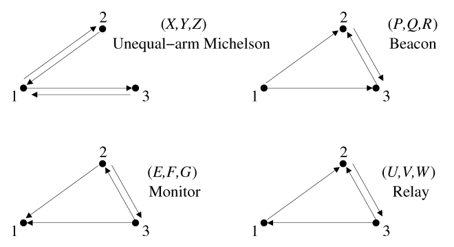
By using the four generators, it is possible to construct several other interferometric combinations, such
as the unequal-arm Michelson  , the Beacons
  , the Monitors
  , and the
Relays
, and the
Relays  . Contrary to the Sagnac combinations, these only use four of the six data
combinations
. Contrary to the Sagnac combinations, these only use four of the six data
combinations  ,
,  . For this reason they have obvious utility in the event of selected subsystem
failures [15*].
. For this reason they have obvious utility in the event of selected subsystem
failures [15*].
These observables can be written in terms of the Sagnac observables  in the following way,
In the case of the combination  , in particular, by writing it in the following form [2*],
![X = [(η1′ + 𝒟2η3) + 𝒟2 𝒟2(η1 + 𝒟3 η2)] − [(η1 + 𝒟3 η2′) + 𝒟3 𝒟3(η1′ + 𝒟2η3)], (46 )](article470x.gif)
 . The first square-bracket term in Eq. (46*) represents a synthesized
light-beam transmitted from spacecraft 1 and made to bounce once at spacecraft 2 and 3,
respectively. The second square-bracket term instead corresponds to another beam also originating
from the same laser, experiencing the same overall delay as the first beam, but bouncing off
spacecraft 3 first and then spacecraft 2. When they are recombined they will cancel the laser phase
fluctuations exactly, having both experienced the same total delay (assuming stationary spacecraft).
The
. The first square-bracket term in Eq. (46*) represents a synthesized
light-beam transmitted from spacecraft 1 and made to bounce once at spacecraft 2 and 3,
respectively. The second square-bracket term instead corresponds to another beam also originating
from the same laser, experiencing the same overall delay as the first beam, but bouncing off
spacecraft 3 first and then spacecraft 2. When they are recombined they will cancel the laser phase
fluctuations exactly, having both experienced the same total delay (assuming stationary spacecraft).
The  combinations should therefore be regarded as the response of a zero-area Sagnac
interferometer.
combinations should therefore be regarded as the response of a zero-area Sagnac
interferometer.
 |
 |
 |
Living Rev. Relativity, 17 (2014), 6, doi:10.12942/lrr-2014-6, URL (accessed <date>): http://www.livingreviews.org/lrr-2014-6.
 This work is licensed under a Creative Commons License.
© The author(s), except where otherwise noted.
This work is licensed under a Creative Commons License.
© The author(s), except where otherwise noted.