Physical and Historical Motivations of TDI

2 Physical and Historical Motivations of TDI

Equal-arm interferometer detectors of gravitational waves can observe gravitational radiation by canceling the laser frequency fluctuations affecting the light injected into their arms. This is done by comparing phases of split beams propagated along the equal (but non-parallel) arms of the detector. The laser frequency fluctuations affecting the two beams experience the same delay within the two equal-length arms and cancel out at the photodetector where relative phases are measured. This way gravitational-wave signals of dimensionless amplitude less than $10−20$ can be observed when using lasers whose frequency stability can be as large as roughly a few parts in $10− 13$ .

If the arms of the interferometer have different lengths, however, the exact cancellation of the laser frequency fluctuations, say $C (t)$ , will no longer take place at the photodetector. In fact, the larger the difference between the two arms, the larger will be the magnitude of the laser frequency fluctuations affecting the detector response. If $L1$ and $L2$ are the lengths of the two arms, it is easy to see that the amount of laser relative frequency fluctuations remaining in the response is equal to (units in which the speed of light $c = 1$ )

In the case of a space-based interferometer such as LISA, whose lasers are expected to display relative frequency fluctuations equal to about $−13 √ --- 10 ∕ Hz$ in the mHz band, and whose arms will differ by a few percent [5 *, 13 , 35 ], Eq. (1 *) implies the following expression for the amplitude of the Fourier components of the uncanceled laser frequency fluctuations (an over-imposed tilde denotes the operation of Fourier transform):

At $f = 10−3 Hz$ , for instance, and assuming $|L − L | ≃ 0.5 s 1 2$ , the uncanceled fluctuations from the laser are equal to $−16 √ --- 6.3 × 10 ∕ Hz$ . Since the LISA sensitivity goal was about $−20 √ --- 10 ∕ Hz$ in this part of the frequency band, it is clear that an alternative experimental approach for canceling the laser frequency fluctuations is needed.

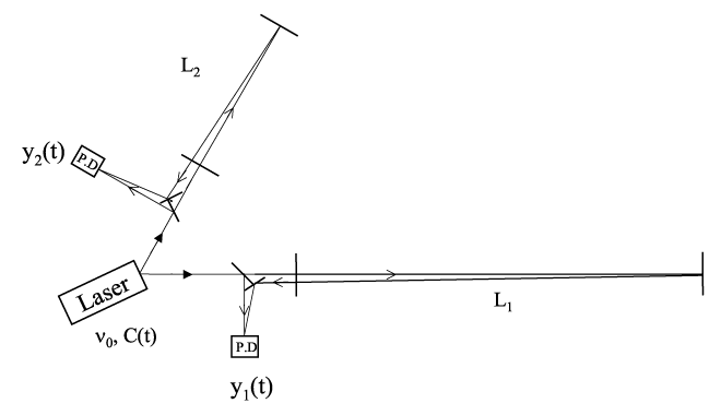
A first attempt to solve this problem was presented by Faller et al. [17 *, 19 , 18 ], and the scheme proposed there can be understood through Figure 1 *. In this idealized model the two beams exiting the two arms are not made to interfere at a common photodetector. Rather, each is made to interfere with the incoming light from the laser at a photodetector, decoupling in this way the phase fluctuations experienced by the two beams in the two arms. Now two Doppler measurements are available in digital form, and the problem now becomes one of identifying an algorithm for digitally canceling the laser frequency fluctuations from a resulting new data combination.

Figure 1: Light from a laser is split into two beams, each injected into an arm formed by pairs of free-falling mirrors. Since the length of the two arms, $L1$ and $L2$ , are different, now the light beams from the two arms are not recombined at one photo detector. Instead each is separately made to interfere with the light that is injected into the arms. Two distinct photo detectors are now used, and phase (or frequency) fluctuations are then monitored and recorded there.

The algorithm they first proposed, and refined subsequently in [24 ], required processing the two Doppler measurements, say $y1(t)$ and $y2(t)$ , in the Fourier domain. If we denote with $h1 (t)$ , $h2(t)$ the gravitational-wave signals entering into the Doppler data $y1$ , $y2$ , respectively, and with $n1$ , $n2$ any other remaining noise affecting $y1$ and $y2$ , respectively, then the expressions for the Doppler observables $y1$ , $y2$ can be written in the following form:

From Eqs. (3 *) and (4 *) it is important to note the characteristic time signature of the random process $C (t)$ in the Doppler responses $y1$ , $y2$ . The time signature of the noise $C(t)$ in $y1(t)$ , for instance, can be understood by observing that the frequency of the signal received at time $t$ contains laser frequency fluctuations transmitted $2L1 s$ earlier. By subtracting from the frequency of the received signal the frequency of the signal transmitted at time $t$ , we also subtract the frequency fluctuations $C(t)$ with the net result shown in Eq. (3 *).

The algorithm for canceling the laser noise in the Fourier domain suggested in [17 ] works as follows. If we take an infinitely long Fourier transform of the data $y 1$ , the resulting expression of $y 1$ in the Fourier domain becomes (see Eq. (3 *))

If the arm length $L1$ is known exactly, we can use the $^y1$ data to estimate the laser frequency fluctuations $C^(f)$ . This can be done by dividing $^y1$ by the transfer function of the laser noise $C$ into the observable $y 1$ itself. By then further multiplying $^y ∕[e4πifL1 − 1] 1$ by the transfer function of the laser noise into the other observable $^y2$ , i.e., $4πifL2 [e − 1]$ , and then subtract the resulting expression from $^y2$ one accomplishes the cancellation of the laser frequency fluctuations.

The problem with this procedure is the underlying assumption of being able to take an infinitely long Fourier transform of the data. Even if one neglects the variation in time of the LISA arms, by taking a finite-length Fourier transform of, say, $y1(t)$ over a time interval $T$ , the resulting transfer function of the laser noise $C$ into $y1$ no longer will be equal to $[e4πifL1 − 1]$ . This can be seen by writing the expression of the finite length Fourier transform of $y1$ in the following way:

where we have denoted with $H (t)$ the function that is equal to 1 in the interval $[− T, +T ]$ , and zero everywhere else. Eq. (6 *) implies that the finite-length Fourier transform $^yT 1$ of $y1(t)$ is equal to the convolution in the Fourier domain of the infinitely long Fourier transform of $y1(t)$ , $^y1$ , with the Fourier transform of $H (t)$ [28 ] (i.e., the “Sinc Function” of width $1 ∕T$ ). The key point here is that we can no longer use the transfer function $[e4πifLi − 1]$ , $i = 1,2$ , for estimating the laser noise fluctuations from one of the measured Doppler data, without retaining residual laser noise into the combination of the two Doppler data $y 1$ , $y 2$ valid in the case of infinite integration time. The amount of residual laser noise remaining in the Fourier-based combination described above, as a function of the integration time $T$ and type of “window function” used, was derived in the appendix of [53 *]. There it was shown that, in order to suppress the residual laser noise below the LISA sensitivity level identified by secondary noises (such as proof-mass and optical path noises) with the use of the Fourier-based algorithm an integration time of about six months was needed.

A solution to this problem was suggested in [53 *], which works entirely in the time-domain. From Eqs. (3 *) and (4 *) we may notice that, by taking the difference of the two Doppler data $y1(t)$ , $y2(t)$ , the frequency fluctuations of the laser now enter into this new data set in the following way:

If we now compare how the laser frequency fluctuations enter into Eq. (7 *) against how they appear in Eqs. (3 *) and (4 *), we can further make the following observation. If we time-shift the data $y (t) 1$ by the round trip light time in arm 2, $y1(t − 2L2)$ , and subtract from it the data $y2(t)$ after it has been time-shifted by the round trip light time in arm 1, $y2(t − 2L1)$ , we obtain the following data set:

In other words, the laser frequency fluctuations enter into $y1(t) − y2(t)$ and $y1(t − 2L2) − y2(t − 2L1)$ with the same time structure. This implies that, by subtracting Eq. (8 *) from Eq. (7 *) we can generate a new data set that does not contain the laser frequency fluctuations $C (t)$ ,

The expression above of the $X$ combination shows that it is possible to cancel the laser frequency noise in the time domain by properly time-shifting and linearly combining Doppler measurements recorded by different Doppler readouts. This in essence is what TDI amounts to.

In order to gain a better physical understanding of how TDI works, let’s rewrite the above $X$ combination in the following form

where we have simply rearranged the terms in Eq. (9 * [45 *].

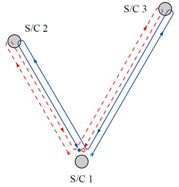
Figure 2: Schematic diagram for $X$ , showing that it is a synthesized zero-area Sagnac interferometer. The optical path begins at an “x” and the measurement is made at an “o”.

Equation (10 *) shows that $X$ is the difference of two sums of relative frequency changes, each corresponding to a specific light path (the continuous and dashed lines in Figure 2 *). The continuous line, corresponding to the first square-bracket term in Eq. (10 *), represents a light-beam transmitted from spacecraft 1 and made to bounce once at spacecraft 3 and 2 respectively. Since the other beam (dashed line) experiences the same overall delay as the first beam (although by bouncing off spacecraft 2 first and then spacecraft 3) when they are recombined they will cancel the laser phase fluctuations exactly, having both experienced the same total delays (assuming stationary spacecraft). For this reason the combination $X$ can be regarded as a synthesized (via TDI) zero-area Sagnac interferometer, with each beam experiencing a delay equal to $(2L + 2L ) 1 2$ . In reality, there are only two beams in each arm (one in each direction) and the lines in Figure 2 * represent the paths of relative frequency changes rather than paths of distinct light beams.

In the following sections we will further elaborate and generalize TDI to the realistic LISA configuration.

	Abstract
1	Introduction
2	Physical and Historical Motivations of TDI
3	Time-Delay Interferometry
4	Algebraic Approach for Canceling Laser and Optical Bench Noises
	4.1	Cancellation of laser phase noise
	4.2	Cancellation of laser phase noise in the unequal-arm interferometer
	4.3	The module of syzygies
	4.4	Gröbner basis
	4.5	Generating set for the module of syzygies
	4.6	Canceling optical bench motion noise
	4.7	Physical interpretation of the TDI combinations
5	Time-Delay Interferometry with Moving Spacecraft
	5.1	The unequal-arm Michelson
	5.2	The Sagnac combinations
	5.3	Algebraic approach to second-generation TDI
	5.4	Solutions with one arm nonfunctional
6	Optimal LISA Sensitivity
	6.1	General application
	6.2	Optimization of SNR for binaries with known direction but with unknown orientation of the orbital plane
7	Experimental Aspects of TDI
	7.1	Time-delays accuracies
	7.2	Clocks synchronization
	7.3	Clocks timing jitter
	7.4	Sampling reconstruction algorithm
	7.5	Data digitization and bit-accuracy requirement
8	Concluding Remarks
	Acknowledgement
A	Generators of the Module of Syzygies
B	Conversion between Generating Sets
	References
	Footnotes
	Updates
	Figures