3 Time-Delay Interferometry
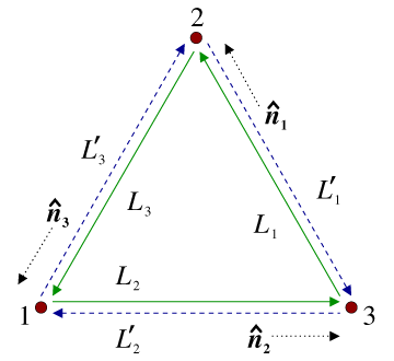
The description of TDI for LISA is greatly simplified if we adopt the notation shown in Figure 3*, where the overall geometry of the LISA detector is defined. There are three spacecraft, six optical benches, six lasers, six proof-masses, and twelve photodetectors. There are also six phase difference data going clock-wise and counter-clockwise around the LISA triangle. For the moment we will make the simplifying assumption that the array is stationary, i.e., the back and forth optical paths between pairs of spacecraft are simply equal to their relative distances [44*, 7*, 45*, 58*]. Several notations have been used in this context. The double index notation recently employed in [45*],
where six quantities are involved, is self-evident. However, when algebraic manipulations are involved the
following notation seems more convenient to use. The spacecraft are labeled 1, 2, 3 and their separating
distances are denoted  ,
,  ,
,  , with
  being opposite spacecraft
  . We orient the vertices 1, 2,
3 clockwise in Figure 3*. Unit vectors between spacecraft are
. We orient the vertices 1, 2,
3 clockwise in Figure 3*. Unit vectors between spacecraft are  , oriented as indicated in
Figure 3*. We index the phase difference data to be analyzed as follows: The beam arriving at
spacecraft
, oriented as indicated in
Figure 3*. We index the phase difference data to be analyzed as follows: The beam arriving at
spacecraft  has subscript
  and is primed or unprimed depending on whether the beam is
traveling clockwise or counter-clockwise (the sense defined here with reference to Figure 3*)
around the LISA triangle, respectively. Thus, as seen from the figure,
and is primed or unprimed depending on whether the beam is
traveling clockwise or counter-clockwise (the sense defined here with reference to Figure 3*)
around the LISA triangle, respectively. Thus, as seen from the figure,  is the phase difference
time series measured at reception at spacecraft 1 with transmission from spacecraft 2 (along
is the phase difference
time series measured at reception at spacecraft 1 with transmission from spacecraft 2 (along
 ).
).
 ,
,  where the index
  corresponds to the opposite spacecraft. The unit
vectors
corresponds to the opposite spacecraft. The unit
vectors  point between pairs of spacecraft, with the orientation indicated.
 Similarly,  is the phase difference series derived from reception at spacecraft 1 with transmission
from spacecraft 3. The other four one-way phase difference time series from signals exchanged between the
spacecraft are obtained by cyclic permutation of the indices:
is the phase difference series derived from reception at spacecraft 1 with transmission
from spacecraft 3. The other four one-way phase difference time series from signals exchanged between the
spacecraft are obtained by cyclic permutation of the indices:  . We also adopt a
notation for delayed data streams, which will be convenient later for algebraic manipulations.
We define the three time-delay operators
. We also adopt a
notation for delayed data streams, which will be convenient later for algebraic manipulations.
We define the three time-delay operators  ,
,  , where for any data stream

 ,
,  , are the light travel times along the three arms of the LISA triangle (the speed of
light
, are the light travel times along the three arms of the LISA triangle (the speed of
light  is assumed to be unity in this article). Thus, for example,
  ,
,
 , etc. Note that the operators commute here. This is because the
arm lengths have been assumed to be constant in time. If the
, etc. Note that the operators commute here. This is because the
arm lengths have been assumed to be constant in time. If the  are functions of time then the operators
no longer commute [7*, 58*], as will be described in Section 4. Six more phase difference series result from
laser beams exchanged between adjacent optical benches within each spacecraft; these are similarly indexed
as
are functions of time then the operators
no longer commute [7*, 58*], as will be described in Section 4. Six more phase difference series result from
laser beams exchanged between adjacent optical benches within each spacecraft; these are similarly indexed
as  ,
,  ,
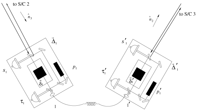
,  . The proof-mass-plus-optical-bench assemblies for LISA spacecraft number 1 are
shown schematically in Figure 4*. The photo receivers that generate the data
. The proof-mass-plus-optical-bench assemblies for LISA spacecraft number 1 are
shown schematically in Figure 4*. The photo receivers that generate the data  ,
,  ,
,  , and
, and  at
spacecraft 1 are shown. The phase fluctuations from the six lasers, which need to be canceled, can be
represented by six random processes
at
spacecraft 1 are shown. The phase fluctuations from the six lasers, which need to be canceled, can be
represented by six random processes  ,
,  , where
  ,
,  are the phases of the lasers in
spacecraft
are the phases of the lasers in
spacecraft  on the left and right optical benches, respectively, as shown in the figure. Note that
this notation is in the same spirit as in [57*, 45*] in which moving spacecraft arrays have been
analyzed.
on the left and right optical benches, respectively, as shown in the figure. Note that
this notation is in the same spirit as in [57*, 45*] in which moving spacecraft arrays have been
analyzed.
We extend the cyclic terminology so that at vertex  ,
,  , the random displacement vectors of
the two proof masses are respectively denoted by
, the random displacement vectors of
the two proof masses are respectively denoted by  ,
,  , and the random displacements (perhaps
several orders of magnitude greater) of their optical benches are correspondingly denoted by
, and the random displacements (perhaps
several orders of magnitude greater) of their optical benches are correspondingly denoted by  ,
,
 where the primed and unprimed indices correspond to the right and left optical benches,
respectively. As pointed out in [15*], the analysis does not assume that pairs of optical benches are rigidly
connected, i.e.,
where the primed and unprimed indices correspond to the right and left optical benches,
respectively. As pointed out in [15*], the analysis does not assume that pairs of optical benches are rigidly
connected, i.e.,  , in general. The present LISA design shows optical fibers transmitting signals
both ways between adjacent benches. We ignore time-delay effects for these signals and will
simply denote by
, in general. The present LISA design shows optical fibers transmitting signals
both ways between adjacent benches. We ignore time-delay effects for these signals and will
simply denote by  the phase fluctuations upon transmission through the fibers of the
laser beams with frequencies
the phase fluctuations upon transmission through the fibers of the
laser beams with frequencies  , and
, and  . The
. The  phase shifts within a given spacecraft
might not be the same for large frequency differences
phase shifts within a given spacecraft
might not be the same for large frequency differences  . For the envisioned frequency
differences (a few hundred MHz), however, the remaining fluctuations due to the optical fiber can be
neglected [15*]. It is also assumed that the phase noise added by the fibers is independent of
the direction of light propagation through them. For ease of presentation, in what follows we
will assume the center frequencies of the lasers to be the same, and denote this frequency by
. For the envisioned frequency
differences (a few hundred MHz), however, the remaining fluctuations due to the optical fiber can be
neglected [15*]. It is also assumed that the phase noise added by the fibers is independent of
the direction of light propagation through them. For ease of presentation, in what follows we
will assume the center frequencies of the lasers to be the same, and denote this frequency by
 .
.
The laser phase noise in  is therefore equal to
  . Similarly, since
  is the phase
shift measured on arrival at spacecraft 2 along arm 1 of a signal transmitted from spacecraft 3, the laser
phase noises enter into it with the following time signature:
is the phase
shift measured on arrival at spacecraft 2 along arm 1 of a signal transmitted from spacecraft 3, the laser
phase noises enter into it with the following time signature:  . Figure 4* endeavors to make
the detailed light paths for these observations clear. An outgoing light beam transmitted to a distant
spacecraft is routed from the laser on the local optical bench using mirrors and beam splitters; this beam
does not interact with the local proof mass. Conversely, an incoming light beam from a distant spacecraft is
bounced off the local proof mass before being reflected onto the photo receiver where it is mixed with light
from the laser on that same optical bench. The inter-spacecraft phase data are denoted
. Figure 4* endeavors to make
the detailed light paths for these observations clear. An outgoing light beam transmitted to a distant
spacecraft is routed from the laser on the local optical bench using mirrors and beam splitters; this beam
does not interact with the local proof mass. Conversely, an incoming light beam from a distant spacecraft is
bounced off the local proof mass before being reflected onto the photo receiver where it is mixed with light
from the laser on that same optical bench. The inter-spacecraft phase data are denoted  and
and  in
Figure 4*.
in
Figure 4*.
 and
and  . The right-hand bench analogously reads
out
. The right-hand bench analogously reads
out  and
and  . The random displacements of the two proof masses and two optical benches are
indicated (lower case
. The random displacements of the two proof masses and two optical benches are
indicated (lower case  for the proof masses, upper case
  for the optical benches).
 Beams between adjacent optical benches within a single spacecraft are bounced off proof masses in the
opposite way. Light to be transmitted from the laser on an optical bench is first bounced off the proof mass
it encloses and then directed to the other optical bench. Upon reception it does not interact with the proof
mass there, but is directly mixed with local laser light, and again down converted. These data are denoted
 and
and  in Figure 4*.
The expressions for the  ,
,  and
and  ,
,  phase measurements can now be developed from
Figures 3* and 4*, and they are for the particular LISA configuration in which all the lasers
have the same nominal frequency
phase measurements can now be developed from
Figures 3* and 4*, and they are for the particular LISA configuration in which all the lasers
have the same nominal frequency  , and the spacecraft are stationary with respect to each
other.1
Consider the
, and the spacecraft are stationary with respect to each
other.1
Consider the  process (Eq. (14*) below). The photo receiver on the right bench of spacecraft 1, which
(in the spacecraft frame) experiences a time-varying displacement
process (Eq. (14*) below). The photo receiver on the right bench of spacecraft 1, which
(in the spacecraft frame) experiences a time-varying displacement  , measures the phase difference
  by first mixing the beam from the distant optical bench 3 in direction
  , and laser phase noise
  and
optical bench motion
and
optical bench motion  that have been delayed by propagation along
  , after one bounce off the
proof mass (
, after one bounce off the
proof mass ( ), with the local laser light (with phase noise
  ). Since for this simplified
configuration no frequency offsets are present, there is of course no need for any heterodyne
conversion [57*].
). Since for this simplified
configuration no frequency offsets are present, there is of course no need for any heterodyne
conversion [57*].
In Eq. (13*) the  measurement results from light originating at the right-bench laser
(
measurement results from light originating at the right-bench laser
( ,
,  ), bounced once off the right proof mass (
 ), and directed through the fiber
(incurring phase shift
), and directed through the fiber
(incurring phase shift  ), to the left bench, where it is mixed with laser light (
 ).
Similarly the right bench records the phase differences
).
Similarly the right bench records the phase differences  and
and  . The laser noises, the
gravitational-wave signals, the optical path noises, and proof-mass and bench noises, enter
into the four data streams recorded at vertex 1 according to the following expressions [15*]:
. The laser noises, the
gravitational-wave signals, the optical path noises, and proof-mass and bench noises, enter
into the four data streams recorded at vertex 1 according to the following expressions [15*]:
![[ ] s = sgw + sopticalpath + 𝒟 p′− p + ν − 2ˆn ⋅⃗δ + nˆ ⋅Δ⃗ + ˆn ⋅ 𝒟 Δ⃗′ , (12 ) 1 1 1 3 2 1 0 3 1 3 1 3 3 2 ′ (⃗′ ⃗ ′) τ1 = p1 − p1 − 2ν0 ˆn2 ⋅ δ1 − Δ 1 + μ1. (13 ) ′ ′gw ′opticalpath ′ [ ⃗′ ⃗′ ⃗ ] s1 = s1 + s1 + 𝒟2p3 − p1 + ν0 2ˆn2 ⋅δ1 − ˆn2 ⋅ Δ1 − ˆn2 ⋅ 𝒟2 Δ3 , (14 ) ′ ′ ( ) τ1 = p1 − p 1 + 2ν0 ˆn3 ⋅ ⃗δ1 − ⃗Δ1 + μ1. (15 )](article210x.gif)
The gravitational-wave phase signal components  ,
,  , in Eqs. (12*) and (14*) are
given by integrating with respect to time the Eqs. (1) and (2) of reference [2*], which relate metric
perturbations to optical frequency shifts. The optical path phase noise contributions
, in Eqs. (12*) and (14*) are
given by integrating with respect to time the Eqs. (1) and (2) of reference [2*], which relate metric
perturbations to optical frequency shifts. The optical path phase noise contributions  ,
,
 , which include shot noise from the low SNR in the links between the distant spacecraft, can be
derived from the corresponding term given in [15*]. The
, which include shot noise from the low SNR in the links between the distant spacecraft, can be
derived from the corresponding term given in [15*]. The  ,
,  measurements will be made with high
SNR so that for them the shot noise is negligible.
measurements will be made with high
SNR so that for them the shot noise is negligible.
 |
 |
 |
Living Rev. Relativity, 17 (2014), 6, doi:10.12942/lrr-2014-6, URL (accessed <date>): http://www.livingreviews.org/lrr-2014-6.
 This work is licensed under a Creative Commons License.
© The author(s), except where otherwise noted.
This work is licensed under a Creative Commons License.
© The author(s), except where otherwise noted.