6 Optimal LISA Sensitivity
All the above interferometric combinations have been shown to individually have rather different sensitivities [15*], as a consequence of their different responses to gravitational radiation and system noises. Since LISA has the capability of simultaneously observing a gravitational-wave signal with many different interferometric combinations (all having different antenna patterns and noises), we should no longer regard LISA as a single detector system but rather as an array of gravitational-wave detectors working in coincidence. This suggests that the LISA sensitivity could be improved by optimally combining elements of the TDI space. Before proceeding with this idea, however, let us consider again the so-called “second-generation” TDI
Sagnac observables:  . The expressions of the gravitational-wave signal and the secondary
noise sources entering into
. The expressions of the gravitational-wave signal and the secondary
noise sources entering into  will in general be different from those entering into
  , the
corresponding Sagnac observable derived under the assumption of a stationary LISA array [2*, 15*].
However, the other remaining, secondary noises in LISA are so much smaller, and the rotation and
systematic velocities in LISA are so intrinsically small, that index permutation may still be done
for them [58*]. It is therefore easy to derive the following relationship between the signal and
secondary noises in
, the
corresponding Sagnac observable derived under the assumption of a stationary LISA array [2*, 15*].
However, the other remaining, secondary noises in LISA are so much smaller, and the rotation and
systematic velocities in LISA are so intrinsically small, that index permutation may still be done
for them [58*]. It is therefore easy to derive the following relationship between the signal and
secondary noises in  , and those entering into the stationary TDI combination
  [45, 58],

 ,
,  , are the unequal-arm lengths of the stationary LISA array. Equation (81*) implies
that any data analysis procedure and algorithm that will be implemented for the second-generation TDI
combinations can actually be derived by considering the corresponding “first-generation” TDI combinations.
For this reason, from now on we will focus our attention on the gravitational-wave responses of the
first-generation TDI observables
, are the unequal-arm lengths of the stationary LISA array. Equation (81*) implies
that any data analysis procedure and algorithm that will be implemented for the second-generation TDI
combinations can actually be derived by considering the corresponding “first-generation” TDI combinations.
For this reason, from now on we will focus our attention on the gravitational-wave responses of the
first-generation TDI observables  .
.
As a consequence of these considerations, we can still regard  as the generators of the TDI
space, and write the most general expression for an element of the TDI space,
as the generators of the TDI
space, and write the most general expression for an element of the TDI space,  , as a linear
combination of the Fourier transforms of the four generators
, as a linear
combination of the Fourier transforms of the four generators  ,
,

 are arbitrary complex functions of the Fourier frequency
  , and of a vector
  containing parameters characterizing the gravitational-wave signal (source location in the sky, waveform
parameters, etc.) and the noises affecting the four responses (noise levels, their correlations, etc.). For a
given choice of the four functions
containing parameters characterizing the gravitational-wave signal (source location in the sky, waveform
parameters, etc.) and the noises affecting the four responses (noise levels, their correlations, etc.). For a
given choice of the four functions  ,
,  gives an element of the functional space of interferometric
combinations generated by
gives an element of the functional space of interferometric
combinations generated by  . Our goal is therefore to identify, for a given gravitational-wave
signal, the four functions
. Our goal is therefore to identify, for a given gravitational-wave
signal, the four functions  that maximize the signal-to-noise ratio
  of the combination
  ,
In Eq. (83*) the subscripts s and n refer to the signal and the noise parts of
,
In Eq. (83*) the subscripts s and n refer to the signal and the noise parts of 
 , respectively, the
angle brackets represent noise ensemble averages, and the interval of integration
, respectively, the
angle brackets represent noise ensemble averages, and the interval of integration  corresponds to
the frequency band accessible by LISA.
corresponds to
the frequency band accessible by LISA.
Before proceeding with the maximization of the  we may notice from Eq. (44*) that the Fourier
transform of the totally symmetric Sagnac combination,
we may notice from Eq. (44*) that the Fourier
transform of the totally symmetric Sagnac combination,  , multiplied by the transfer function
 can be written as a linear combination of the Fourier transforms of the remaining three
generators
can be written as a linear combination of the Fourier transforms of the remaining three
generators  . Since the signal-to-noise ratio of
  and
and  are equal, we may
conclude that the optimization of the signal-to-noise ratio of
are equal, we may
conclude that the optimization of the signal-to-noise ratio of  can be performed only on
the three observables
can be performed only on
the three observables  . This implies the following redefined expression for
  :
:
 can be regarded as a functional over the space of the three complex functions
  , and
the particular set of complex functions that extremize it can of course be derived by solving the associated
set of Euler–Lagrange equations.
, and
the particular set of complex functions that extremize it can of course be derived by solving the associated
set of Euler–Lagrange equations.
In order to make the derivation of the optimal SNR easier, let us first denote by  and
and  the
two vectors of the signals
the
two vectors of the signals  and the noises
  , respectively. Let us also define
  to
be the vector of the three functions
to
be the vector of the three functions  , and denote with
  the Hermitian, non-singular, correlation
matrix of the vector random process
the Hermitian, non-singular, correlation
matrix of the vector random process  ,
,

 to be the components of the Hermitian matrix
  , we can rewrite
 in the following form,
where we have adopted the usual convention of summation over repeated indices. Since the noise correlation
matrix
in the following form,
where we have adopted the usual convention of summation over repeated indices. Since the noise correlation
matrix 
 is non-singular, and the integrand is positive definite or null, the stationary values of
the signal-to-noise ratio will be attained at the stationary values of the integrand, which are
given by solving the following set of equations (and their complex conjugated expressions):
After taking the partial derivatives, Eq. (87*) can be rewritten in the following form,
which tells us that the stationary values of the signal-to-noise ratio of
is non-singular, and the integrand is positive definite or null, the stationary values of
the signal-to-noise ratio will be attained at the stationary values of the integrand, which are
given by solving the following set of equations (and their complex conjugated expressions):
After taking the partial derivatives, Eq. (87*) can be rewritten in the following form,
which tells us that the stationary values of the signal-to-noise ratio of ![[ aA a∗] -∂-- --i-ij-j = 0, k = 1,2, 3. (87 ) ∂ak arCrta ∗t](article731x.gif)
![[ ∗ ] (C − 1)ir (A )rj (a∗)j = apApqa-q (a∗)i, i = 1,2,3, (88 ) alClma ∗m](article732x.gif)
 are equal to the eigenvalues of the
the matrix
are equal to the eigenvalues of the
the matrix  . The result in Eq. (87*) is well known in the theory of quadratic forms, and it is called
Rayleigh’s principle [36, 42].
. The result in Eq. (87*) is well known in the theory of quadratic forms, and it is called
Rayleigh’s principle [36, 42].
In order now to identify the eigenvalues of the matrix  , we first notice that the
  matrix
 has rank 1. This implies that the matrix
  has also rank 1, as it is easy to verify. Therefore
two of its three eigenvalues are equal to zero, while the remaining non-zero eigenvalue represents the
solution we are looking for.
has also rank 1, as it is easy to verify. Therefore
two of its three eigenvalues are equal to zero, while the remaining non-zero eigenvalue represents the
solution we are looking for.
The analytic expression of the third eigenvalue can be obtained by using the property that the trace of
the  matrix
  is equal to the sum of its three eigenvalues, and in our case to the eigenvalue
we are looking for. From these considerations we derive the following expression for the optimized
signal-to-noise ratio
is equal to the sum of its three eigenvalues, and in our case to the eigenvalue
we are looking for. From these considerations we derive the following expression for the optimized
signal-to-noise ratio  :
:

- Among all possible interferometric combinations LISA will be able to synthesize with its four
generators
 ,
,  ,
,  ,
,  , the particular combination giving maximum signal-to-noise ratio
can be obtained by using only three of them, namely
, the particular combination giving maximum signal-to-noise ratio
can be obtained by using only three of them, namely  .
.
- The expression of the optimal signal-to-noise ratio given by Eq. (89*) implies that LISA
should be regarded as a network of three interferometer detectors of gravitational radiation (of
responses
 ) working in coincidence [20, 40*].
6.1 General application
As an application of Eq. (89*), here we calculate the sensitivity that LISA can reach when observing
sinusoidal signals uniformly distributed on the celestial sphere and of random polarization. In order to
calculate the optimal signal-to-noise ratio we will also need to use a specific expression for the noise
correlation matrix  . As a simplification, we will assume the LISA arm lengths to be equal to
their nominal value
. As a simplification, we will assume the LISA arm lengths to be equal to
their nominal value  , the optical-path noises to be equal and uncorrelated to
each other, and finally the noises due to the proof-mass noises to be also equal, uncorrelated
to each other and to the optical-path noises. Under these assumptions the correlation matrix
becomes real, its three diagonal elements are equal, and all the off-diagonal terms are equal to
each other, as it is easy to verify by direct calculation [15*]. The noise correlation matrix
, the optical-path noises to be equal and uncorrelated to
each other, and finally the noises due to the proof-mass noises to be also equal, uncorrelated
to each other and to the optical-path noises. Under these assumptions the correlation matrix
becomes real, its three diagonal elements are equal, and all the off-diagonal terms are equal to
each other, as it is easy to verify by direct calculation [15*]. The noise correlation matrix  is therefore uniquely identified by two real functions
  and
and  in the following way:
The expression of the optimal signal-to-noise ratio assumes a rather simple form if we diagonalize this
correlation matrix by properly “choosing a new basis”. There exists an orthogonal transformation
of the generators  , which will transform the optimal signal-to-noise ratio into the
sum of the signal-to-noise ratios of the “transformed” three interferometric combinations. The
expressions of the three eigenvalues
, which will transform the optimal signal-to-noise ratio into the
sum of the signal-to-noise ratios of the “transformed” three interferometric combinations. The
expressions of the three eigenvalues  (which are real) of the noise correlation matrix
  can easily be found by using the algebraic manipulator Mathematica, and they are equal to

 ,
,  ), are equal. This implies that the eigenvector
associated to
), are equal. This implies that the eigenvector
associated to  is orthogonal to the two-dimensional space generated by the eigenvalue
  , while any
chosen pair of eigenvectors corresponding to
, while any
chosen pair of eigenvectors corresponding to  will not necessarily be orthogonal. This inconvenience can
be avoided by choosing an arbitrary set of vectors in this two-dimensional space, and by ortho-normalizing
them. After some simple algebra, we have derived the following three ortho-normalized eigenvectors:
Equation (92*) implies the following three linear combinations of the generators
will not necessarily be orthogonal. This inconvenience can
be avoided by choosing an arbitrary set of vectors in this two-dimensional space, and by ortho-normalizing
them. After some simple algebra, we have derived the following three ortho-normalized eigenvectors:
Equation (92*) implies the following three linear combinations of the generators 
 :
where
:
where 
 ,
,  , and
, and  are italicized to indicate that these are “orthogonal modes”. Although the
expressions for the modes
are italicized to indicate that these are “orthogonal modes”. Although the
expressions for the modes  and
and  depend on our particular choice for the two eigenvectors (
 ),
it is clear from our earlier considerations that the value of the optimal signal-to-noise ratio is unaffected by
such a choice. From Eq. (93*) it is also easy to verify that the noise correlation matrix of these three
combinations is diagonal, and that its non-zero elements are indeed equal to the eigenvalues given in
Eq. (91*).
),
it is clear from our earlier considerations that the value of the optimal signal-to-noise ratio is unaffected by
such a choice. From Eq. (93*) it is also easy to verify that the noise correlation matrix of these three
combinations is diagonal, and that its non-zero elements are indeed equal to the eigenvalues given in
Eq. (91*).
In order to calculate the sensitivity corresponding to the expression of the optimal signal-to-noise ratio,
we have proceeded similarly to what was done in [2*, 15*], and described in more detail in [56*]. We assume
an equal-arm LISA ( ), and take the one-sided spectra of proof mass and aggregate
optical-path-noises (on a single link), expressed as fractional frequency fluctuation spectra, to be
), and take the one-sided spectra of proof mass and aggregate
optical-path-noises (on a single link), expressed as fractional frequency fluctuation spectra, to be
![S pyroofmass= 2.5 × 10 −48[f∕1 Hz ]−2 Hz− 1](article774x.gif) and
and ![Syopticalpath = 1.8 × 10−37[f ∕1 Hz]2 Hz− 1](article775x.gif) , respectively (see
[15*, 5]). We also assume that aggregate optical path noise has the same transfer function as shot
noise.
, respectively (see
[15*, 5]). We also assume that aggregate optical path noise has the same transfer function as shot
noise.
The optimum SNR is the square root of the sum of the squares of the SNRs of the three “orthogonal
modes”  . To compare with previous sensitivity curves of a single LISA Michelson interferometer,
we construct the SNRs as a function of Fourier frequency for sinusoidal waves from sources uniformly
distributed on the celestial sphere. To produce the SNR of each of the
. To compare with previous sensitivity curves of a single LISA Michelson interferometer,
we construct the SNRs as a function of Fourier frequency for sinusoidal waves from sources uniformly
distributed on the celestial sphere. To produce the SNR of each of the  modes we need the
gravitational-wave response and the noise response as a function of Fourier frequency. We build up the
gravitational-wave responses of the three modes
modes we need the
gravitational-wave response and the noise response as a function of Fourier frequency. We build up the
gravitational-wave responses of the three modes  from the gravitational-wave responses of
 . For 7000 Fourier frequencies in the
  to
to  LISA band, we produce the
Fourier transforms of the gravitational-wave response of
LISA band, we produce the
Fourier transforms of the gravitational-wave response of  from the formulas in [2*, 56]. The
averaging over source directions (uniformly distributed on the celestial sphere) and polarization states
(uniformly distributed on the Poincaré sphere) is performed via a Monte Carlo method. From
the Fourier transforms of the
from the formulas in [2*, 56]. The
averaging over source directions (uniformly distributed on the celestial sphere) and polarization states
(uniformly distributed on the Poincaré sphere) is performed via a Monte Carlo method. From
the Fourier transforms of the  responses at each frequency, we construct the Fourier
transforms of
responses at each frequency, we construct the Fourier
transforms of  . We then square and average to compute the mean-squared responses of
 at that frequency from
  realizations of (source position, polarization state)
pairs.
realizations of (source position, polarization state)
pairs.
We adopt the following terminology: We refer to a single element of the module as a data combination, while a function of the elements of the module, such as taking the maximum over several data combinations in the module or squaring and adding data combinations belonging to the module, is called as an observable. The important point to note is that the laser frequency noise is also suppressed for the observable although it may not be an element of the module.
The noise spectra of  are determined from the raw spectra of proof-mass and optical-path
noises, and the transfer functions of these noises to
are determined from the raw spectra of proof-mass and optical-path
noises, and the transfer functions of these noises to  . Using the transfer functions given in [15*],
the resulting spectra are equal to
. Using the transfer functions given in [15*],
the resulting spectra are equal to
![S (f) = S (f) = 16 sin2(πf L) [3 + 2 cos(2 πfL ) + cos(4πf L )]Sproof mass(f ) A E y +8 sin2(πfL )[2 + cos(2πfL )]Syopticalpath(f), (94 ) 2[ 2 proofmass opticalpath ] ST (f) = 2[1 + 2cos(2πf L)] 4 sin (πf L) Sy + Sy (f) . (95 )](article789x.gif)
 . The SNR for, e.g.,
  ,
,  , at each
frequency
, at each
frequency  is equal to
  times the ratio of the root-mean-squared gravitational-wave response at that
frequency divided by
times the ratio of the root-mean-squared gravitational-wave response at that
frequency divided by  , where
  is the bandwidth conventionally taken to be equal to 1 cycle
per year. Finally, if we take the reciprocal of
is the bandwidth conventionally taken to be equal to 1 cycle
per year. Finally, if we take the reciprocal of  and multiply it by 5 to get the conventional
 sensitivity criterion, we obtain the sensitivity curve for this combination, which
can then be compared against the corresponding sensitivity curve for the equal-arm Michelson
interferometer.
sensitivity criterion, we obtain the sensitivity curve for this combination, which
can then be compared against the corresponding sensitivity curve for the equal-arm Michelson
interferometer.
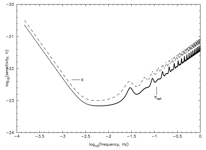
In Figure 7* we show the sensitivity curve for the LISA equal-arm Michelson response ( ) as a
function of the Fourier frequency, and the sensitivity curve from the optimum weighting of the data
described above:
) as a
function of the Fourier frequency, and the sensitivity curve from the optimum weighting of the data
described above:  . The SNRs were computed for a bandwidth of 1
cycle/year. Note that at frequencies where the LISA Michelson combination has best sensitivity, the
improvement in signal-to-noise ratio provided by the optimal observable is slightly larger than
. The SNRs were computed for a bandwidth of 1
cycle/year. Note that at frequencies where the LISA Michelson combination has best sensitivity, the
improvement in signal-to-noise ratio provided by the optimal observable is slightly larger than
 .
.
 = 16.67 s.
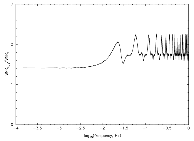
 . The sensitivity gain in the low-frequency band is equal to
  , while
it can get larger than 2 at selected frequencies in the high-frequency region of the accessible band.
The integration time has been assumed to be one year, and the proof mass and optical path noise
spectra are the nominal ones. See the main body of the paper for a quantitative discussion of this
point.
, while
it can get larger than 2 at selected frequencies in the high-frequency region of the accessible band.
The integration time has been assumed to be one year, and the proof mass and optical path noise
spectra are the nominal ones. See the main body of the paper for a quantitative discussion of this
point.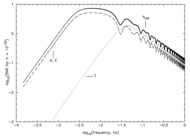
 and their sum as a function of the Fourier
frequency
and their sum as a function of the Fourier
frequency  . The SNRs of
  and
and  are equal over the entire frequency band. The SNR of
  is significantly smaller than the other two in the low part of the frequency band, while is comparable
to (and at times larger than) the SNR of the other two in the high-frequency region. See text for a
complete discussion.
is significantly smaller than the other two in the low part of the frequency band, while is comparable
to (and at times larger than) the SNR of the other two in the high-frequency region. See text for a
complete discussion. In Figure 8* we plot the ratio between the optimal SNR and the SNR of a single Michelson
interferometer. In the long-wavelength limit, the SNR improvement is  . For Fourier frequencies greater
than or about equal to
. For Fourier frequencies greater
than or about equal to  , the SNR improvement is larger and varies with the frequency, showing an
average value of about
, the SNR improvement is larger and varies with the frequency, showing an
average value of about  . In particular, for bands of frequencies centered on integer multiples of
 ,
,  contributes strongly and the aggregate SNR in these bands can be greater than
2.
contributes strongly and the aggregate SNR in these bands can be greater than
2.
In order to better understand the contribution from the three different combinations to the optimal
combination of the three generators, in Figure 9* we plot the signal-to-noise ratios of  as well as
the optimal signal-to-noise ratio. For an assumed
as well as
the optimal signal-to-noise ratio. For an assumed  , the SNRs of the three modes are plotted
versus frequency. For the equal-arm case computed here, the SNRs of
, the SNRs of the three modes are plotted
versus frequency. For the equal-arm case computed here, the SNRs of  and
and  are equal across the
band. In the long wavelength region of the band, modes
are equal across the
band. In the long wavelength region of the band, modes  and
and  have SNRs much greater than mode
 , where its contribution to the total SNR is negligible. At higher frequencies, however, the
 combination has SNR greater than or comparable to the other modes and can dominate
the SNR improvement at selected frequencies. Some of these results have also been obtained
in [40*].
combination has SNR greater than or comparable to the other modes and can dominate
the SNR improvement at selected frequencies. Some of these results have also been obtained
in [40*].
6.2 Optimization of SNR for binaries with known direction but with unknown orientation of the orbital plane
Binaries are important sources for LISA and therefore the analysis of such sources is of major importance.
One such class is of massive or super-massive binaries whose individual masses could range from  to
to  and which could be up to a few Gpc away. Another class of interest are known binaries within
our own galaxy whose individual masses are of the order of a solar mass but are just at a distance of a few
kpc or less. Here the focus will be on this latter class of binaries. It is assumed that the direction of the
source is known, which is so for known binaries in our galaxy. However, even for such binaries, the
inclination angle of the plane of the orbit of the binary is either poorly estimated or unknown. The
optimization problem is now posed differently: The SNR is optimized after averaging over the
polarizations of the binary signals, so the results obtained are optimal on the average, that is, the
source is tracked with an observable which is optimal on the average [40*]. For computing the
average, a uniform distribution for the direction of the orbital angular momentum of the binary is
assumed.
and which could be up to a few Gpc away. Another class of interest are known binaries within
our own galaxy whose individual masses are of the order of a solar mass but are just at a distance of a few
kpc or less. Here the focus will be on this latter class of binaries. It is assumed that the direction of the
source is known, which is so for known binaries in our galaxy. However, even for such binaries, the
inclination angle of the plane of the orbit of the binary is either poorly estimated or unknown. The
optimization problem is now posed differently: The SNR is optimized after averaging over the
polarizations of the binary signals, so the results obtained are optimal on the average, that is, the
source is tracked with an observable which is optimal on the average [40*]. For computing the
average, a uniform distribution for the direction of the orbital angular momentum of the binary is
assumed.
When the binary masses are of the order of a solar mass and the signal typically has a frequency of a few mHz, the GW frequency of the binary may be taken to be constant over the period of observation, which is typically taken to be of the order of an year. A complete calculation of the signal matrix and the optimization procedure of SNR is given in [39*]. Here we briefly mention the main points and the final results.
A source fixed in the Solar System Barycentric reference frame in the direction  is considered.
But as the LISA constellation moves along its heliocentric orbit, the apparent direction
is considered.
But as the LISA constellation moves along its heliocentric orbit, the apparent direction  of the
source in the LISA reference frame
of the
source in the LISA reference frame  changes with time. The LISA reference frame
  has been defined in [39*] as follows: The origin lies at the center of the LISA triangle and the plane of LISA
coincides with the
has been defined in [39*] as follows: The origin lies at the center of the LISA triangle and the plane of LISA
coincides with the  plane with spacecraft 2 lying on the
  axis. Figure (10*) displays this
apparent motion for a source lying in the ecliptic plane, that is with
axis. Figure (10*) displays this
apparent motion for a source lying in the ecliptic plane, that is with  and
and  . The source
in the LISA reference frame describes a figure of 8. Optimizing the SNR amounts to tracking
the source with an optimal observable as the source apparently moves in the LISA reference
frame.
. The source
in the LISA reference frame describes a figure of 8. Optimizing the SNR amounts to tracking
the source with an optimal observable as the source apparently moves in the LISA reference
frame.
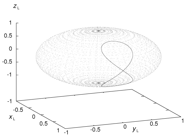
 . The track of the source for a period of one year is shown on the unit sphere
in the LISA reference frame.
. The track of the source for a period of one year is shown on the unit sphere
in the LISA reference frame. Since an average has been taken over the orientation of the orbital plane of the binary or equivalently
over the polarizations, the signal matrix  is now of rank 2 instead of rank 1 as compared with
the application in the previous Section 6.1. The mutually orthogonal data combinations
is now of rank 2 instead of rank 1 as compared with
the application in the previous Section 6.1. The mutually orthogonal data combinations  ,
,
 ,
,  are convenient in carrying out the computations because in this case as well, they
simultaneously diagonalize the signal and the noise covariance matrix. The optimization problem now
reduces to an eigenvalue problem with the eigenvalues being the squares of the SNRs. There
are two eigen-vectors which are labeled as
are convenient in carrying out the computations because in this case as well, they
simultaneously diagonalize the signal and the noise covariance matrix. The optimization problem now
reduces to an eigenvalue problem with the eigenvalues being the squares of the SNRs. There
are two eigen-vectors which are labeled as  belonging to two non-zero eigenvalues. The
two SNRs are labelled as
belonging to two non-zero eigenvalues. The
two SNRs are labelled as  and
and  , corresponding to the two orthogonal (thus
statistically independent) eigenvectors
, corresponding to the two orthogonal (thus
statistically independent) eigenvectors  . As was done in the previous Section 6.1 F the two
SNRs can be squared and added to yield a network SNR, which is defined through the equation
. As was done in the previous Section 6.1 F the two
SNRs can be squared and added to yield a network SNR, which is defined through the equation

 and
and  gives zero signal.
The eigenvectors and the SNRs are functions of the apparent source direction parameters  in
the LISA reference frame, which in turn are functions of time. The eigenvectors optimally track the
source as it moves in the LISA reference frame. Assuming an observation period of an year, the
SNRs are integrated over this period of time. The sensitivities are computed according to the
procedure described in the previous Section 6.1. The results of these findings are displayed in
Figure 11*.
in
the LISA reference frame, which in turn are functions of time. The eigenvectors optimally track the
source as it moves in the LISA reference frame. Assuming an observation period of an year, the
SNRs are integrated over this period of time. The sensitivities are computed according to the
procedure described in the previous Section 6.1. The results of these findings are displayed in
Figure 11*.
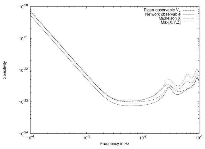
It shows the sensitivity curves of the following observables:
- The Michelson combination
 (faint solid curve).
- The observable obtained by taking the maximum sensitivity among
 ,
,  , and
, and  for each
direction, where
for each
direction, where  and
and  are the Michelson observables corresponding to the remaining
two pairs of arms of LISA [2]. This maximum is denoted by
are the Michelson observables corresponding to the remaining
two pairs of arms of LISA [2]. This maximum is denoted by ![max [X, Y, Z]](article856x.gif) (dash-dotted curve)
and is operationally given by switching the combinations
(dash-dotted curve)
and is operationally given by switching the combinations  ,
,  ,
,  so that the best
sensitivity is achieved.
so that the best
sensitivity is achieved.
- The eigen-combination
 which has the best sensitivity among all data combinations (dashed
curve).
which has the best sensitivity among all data combinations (dashed
curve).
- The network observable (solid curve).
It is observed that the sensitivity over the band-width of LISA increases as one goes from
Observable 1 to 4. Also it is seen that the ![max [X, Y, Z]](article861x.gif) does not do much better than
does not do much better than  . This
is because for the source direction chosen
. This
is because for the source direction chosen  ,
,  is reasonably well oriented and
switching to
is reasonably well oriented and
switching to  and
and  combinations does not improve the sensitivity significantly. However, the
network and
combinations does not improve the sensitivity significantly. However, the
network and  observables show significant improvement in sensitivity over both
  and
and
![max [X, Y,Z ]](article869x.gif) . This is the typical behavior and the sensitivity curves (except
. This is the typical behavior and the sensitivity curves (except  ) do not show much
variations for other source directions and the plots are similar. Also it may be fair to compare the
optimal sensitivities with
) do not show much
variations for other source directions and the plots are similar. Also it may be fair to compare the
optimal sensitivities with ![max [X,Y, Z ]](article871x.gif) rather than
rather than  . This comparison of sensitivities is
shown in Figure 12*, where the network and the eigen-combinations
. This comparison of sensitivities is
shown in Figure 12*, where the network and the eigen-combinations  are compared with
![max [X, Y,Z ]](article874x.gif) .
.
![max [X, Y,Z ]](article876x.gif) ,
,  , and network for
the source direction (
, and network for
the source direction ( ,
,  ).
).
 with
with ![max [X, Y,Z ]](article882x.gif) for the
source direction
for the
source direction  ,
,  .
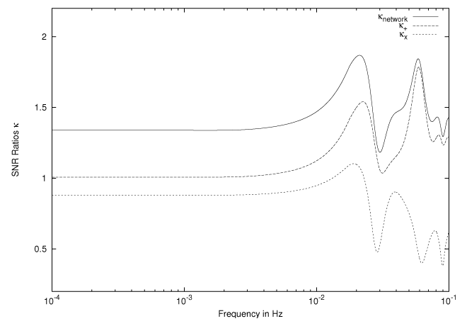
.Defining
where the subscript](article885x.gif)
 stands for network or
  ,
,  , and
, and ![SNRmax [X,Y,Z]](article889x.gif) is the SNR of the observable
is the SNR of the observable
![max [X, Y,Z ]](article890x.gif) , the ratios of sensitivities are plotted over the LISA band-width. The improvement in
sensitivity for the network observable is about 34% at low frequencies and rises to nearly 90% at about
20 mHz, while at the same time the
, the ratios of sensitivities are plotted over the LISA band-width. The improvement in
sensitivity for the network observable is about 34% at low frequencies and rises to nearly 90% at about
20 mHz, while at the same time the  combination shows improvement of 12% at low frequencies rising
to over 50% at about 20 mHz.
combination shows improvement of 12% at low frequencies rising
to over 50% at about 20 mHz.
 |
 |
 |
Living Rev. Relativity, 17 (2014), 6, doi:10.12942/lrr-2014-6, URL (accessed <date>): http://www.livingreviews.org/lrr-2014-6.
 This work is licensed under a Creative Commons License.
© The author(s), except where otherwise noted.
This work is licensed under a Creative Commons License.
© The author(s), except where otherwise noted.