List of Figures
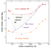 |
Figure 1:
Endpoints of evolution of moderate-mass nonrotating single stars depending on initial mass and metallicity. Image reproduced with permission from [709], copyright by IAU. |
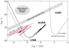 |
Figure 2:
Sensitivity limits of GW detectors and the regions of the  – – diagram occupied by
some potential GW sources. (Courtesy G. Nelemans). diagram occupied by
some potential GW sources. (Courtesy G. Nelemans). |
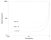 |
Figure 3:
The maximum initial orbital period (in hours) of two point masses that will coalesce due to gravitational wave emission in a time interval shorter than 1010 yr, as a function of the initial eccentricity  . The lines are calculated for . The lines are calculated for  (BH + BH), (BH + BH),  (BH + NS), and
  (NS + NS). (NS + NS). |
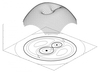 |
Figure 4:
A 3-D representation of a dimensionless Roche potential in the co-rotating frame for a binary with a mass ratio of components  . . |
 |
Figure 5:
Descendants of components of close binaries depending on the radius of the star at RLOF. The upper solid line separates close and wide binaries (after [293]). The boundary between progenitors of He- and CO-WDs is uncertain by several  , the boundary between CO and ONe varieties
of WDs and WD and NSs – by , the boundary between CO and ONe varieties
of WDs and WD and NSs – by  . The boundary between progenitors of NS and BH is shown
at . The boundary between progenitors of NS and BH is shown
at  after [643], while it may be possible that it really is between after [643], while it may be possible that it really is between  and and  (see
Section 1 for discussion and references.) (see
Section 1 for discussion and references.) |
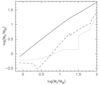 |
Figure 6:
Relation between ZAMS masses of stars  and their masses at TAMS (solid line),
masses of helium stars (dashed line), masses of He WD (dash-dotted line), masses of CO and ONe
WD (dotted line). For stars with and their masses at TAMS (solid line),
masses of helium stars (dashed line), masses of He WD (dash-dotted line), masses of CO and ONe
WD (dotted line). For stars with  we plot the upper limit of WD masses for case B of
mass exchange. After [791]. we plot the upper limit of WD masses for case B of
mass exchange. After [791]. |
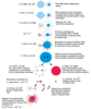 |
Figure 7:
Evolutionary scenario for the formation of neutron stars or black holes in close binaries. T is the typical time scale of an evolutionary stage, N is the estimated number of objects in the given evolutionary stage. |
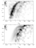 |
Figure 8:
Upper panel: the probability distribution for the orbital parameters of the NS + NS binaries with  day at the moment of birth. The darkest shade corresponds to a birthrate of day at the moment of birth. The darkest shade corresponds to a birthrate of
 . Lower panel: the probability distribution for the present-day orbital parameters
of the Galactic disc NS + NS binaries younger than 10 Gyr. The grey scaling represents numbers in
the Galaxy. The darkest shade corresponds to 1100 binaries with given combination of . Lower panel: the probability distribution for the present-day orbital parameters
of the Galactic disc NS + NS binaries younger than 10 Gyr. The grey scaling represents numbers in
the Galaxy. The darkest shade corresponds to 1100 binaries with given combination of  and and
 . . |
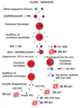 |
Figure 9:
Formation of close dwarf binaries and their descendants (scale and color-coding are arbitrary). |
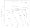 |
Figure 10:
Limits of different burning regimes of accreted hydrogen onto a CO WD as a function of mass of the WD and accretion rate  [535]. If [535]. If 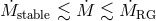 , hydrogen burns steadily.
If , hydrogen burns steadily.
If  , H-burning shells are thermally unstable; with decrease of , H-burning shells are thermally unstable; with decrease of  the strength of
flashes increases. For the strength of
flashes increases. For  , hydrogen burns steadily but the excess of unburnt matter forms
an extended red-giant–sized envelope. In the latter case white dwarfs may lose matter by wind or
due to Roche lobe overflow. A dotted line shows the Eddington accretion rate , hydrogen burns steadily but the excess of unburnt matter forms
an extended red-giant–sized envelope. In the latter case white dwarfs may lose matter by wind or
due to Roche lobe overflow. A dotted line shows the Eddington accretion rate  as a function
of as a function
of  . The dashed lines are the loci of the hydrogen envelope mass at hydrogen ignition. Image
reproduced with permission from [535], copyright by AAS. . The dashed lines are the loci of the hydrogen envelope mass at hydrogen ignition. Image
reproduced with permission from [535], copyright by AAS. |
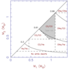 |
Figure 11:
Possible combinations of masses and chemical compositions of components in a close WD binary [461]. Solid curves are lines of constant chirp mass (see Sections 3.1.2 and 10). Image reproduced with permission from [461], copyright by IOP. |
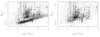 |
Figure 12:
The total masses of binaries in the simulated population of WD binaries with  as a function of system’s orbital period. In the left plot the outcome of the first common envelope
stage is described by
as a function of system’s orbital period. In the left plot the outcome of the first common envelope
stage is described by  -formalism, Eq. (59*), and in the right plot – by -formalism, Eq. (59*), and in the right plot – by  -formalism, Eq. (57*). In
both plots the latter equation describes both common envelope stages. The grey scale (the same for
both plots) corresponds to the density of objects in the linear scale. Observed WD binaries are shown
as filled circles (see the original paper for references). The Chandrasekhar mass limit is shown by
the dotted line. To the left of the dashed line the systems merge within 13.5 Gyr. Image reproduced
with permission from [766], copyright by ESO. -formalism, Eq. (57*). In
both plots the latter equation describes both common envelope stages. The grey scale (the same for
both plots) corresponds to the density of objects in the linear scale. Observed WD binaries are shown
as filled circles (see the original paper for references). The Chandrasekhar mass limit is shown by
the dotted line. To the left of the dashed line the systems merge within 13.5 Gyr. Image reproduced
with permission from [766], copyright by ESO. |
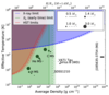 |
Figure 13:
Constraints on mass, effective temperature, radius and average density of the primary star of SN 2011fe. The shaded red region is excluded by non-detection of an optical quiescent counterpart in the Hubble Space Telescope imaging. The shaded green region is excluded from considerations of the non-detection of a shock breakout at early times. The blue region is excluded by the non-detection of a quiescent counterpart in the Chandra X-ray imaging. The location of the H, He, and C main-sequence is shown, with the symbol size scaled for different primary masses. Several observed WDs and NSs are shown. The primary radius in units of  is shown for mass is shown for mass
 . Image reproduced with permission from [57], copyright by AAS. . Image reproduced with permission from [57], copyright by AAS. |
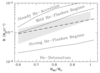 |
Figure 14:
Limits on different burning regimes of helium accreted onto a CO WD as a function of the WD mass and accretion rate [590], Piersanti, Tornambé & Yungelson (in prep.). Above the “RG Configuration” line, accreted He forms an extended red-giant–like envelope. Below  , accreted He detonates and the mass is lost dynamically. In the strong-flashes
regime, He-layer expands and mass is lost due to RLOF and interaction with the companion. Helium
accumulation efficiency for this regime is shown in Figure 15, and the critical He masses for WD
detonation are shown in Figure 28. Shaded region shows the domain of stable burning of accreted
hydrogen. , accreted He detonates and the mass is lost dynamically. In the strong-flashes
regime, He-layer expands and mass is lost due to RLOF and interaction with the companion. Helium
accumulation efficiency for this regime is shown in Figure 15, and the critical He masses for WD
detonation are shown in Figure 28. Shaded region shows the domain of stable burning of accreted
hydrogen. |
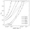 |
Figure 15:
The accumulation efficiency of helium as a function of the accretion rate for CO WD models of 0.6, 0.7, 0.81, 0.92,  (top to bottom), as calculated by Piersanti et al. (in prep.).
Dotted and dashed lines represent the accumulation efficiency for CO WDs with initial masses 0.9
and (top to bottom), as calculated by Piersanti et al. (in prep.).
Dotted and dashed lines represent the accumulation efficiency for CO WDs with initial masses 0.9
and  , respectively, after Kato & Hachisu [347]. , respectively, after Kato & Hachisu [347]. |
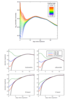 |
Figure 16:
Upper panel: model light curve of a SN Ia having collided with a red giant companion separated by  . The luminosity due to the collision is prominent at times . The luminosity due to the collision is prominent at times  days.
The black dashed line shows the analytic prediction for the early phase luminosity. Lower panel:
Signatures of interaction in the early broadband light curves of SN Ia for a red-giant companion at days.
The black dashed line shows the analytic prediction for the early phase luminosity. Lower panel:
Signatures of interaction in the early broadband light curves of SN Ia for a red-giant companion at
 (green lines), a (green lines), a  main-sequence companion at main-sequence companion at  (blue lines), and
a (blue lines), and
a  main-sequence companion at main-sequence companion at  (red lines). The ultraviolet light curves are
constructed by integrating the flux in the region 1000 – 3000 Å and converting to the AB magnitude
system. For all light curves shown, the viewing angle is 0. Image reproduced with permission
from [340], copyright by AAS. (red lines). The ultraviolet light curves are
constructed by integrating the flux in the region 1000 – 3000 Å and converting to the AB magnitude
system. For all light curves shown, the viewing angle is 0. Image reproduced with permission
from [340], copyright by AAS. |
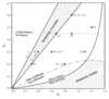 |
Figure 17:
Estimates of regimes of mass transfer in WD binaries. Instantaneous tidal coupling is assumed. For longer time scales of tidal coupling, the stability limit in the plot shifts down [464]. The filled squares mark initial positions of the models studied in the quoted paper. Image reproduced with permission from [129], copyright by AAS. |
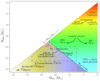 |
Figure 18:
Outcomes of merger of WD binaries depending on the mass and chemical composition of the components. Systems in the hatched region are expected to experience He-detonations during mass transfer or at the time of merger. The numbers near the arrows indicate relevant timescales. Image reproduced with permission from Figure 1 of [128], copyright by the authors. |
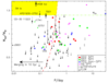 |
Figure 19:
Known close binaries with two WD components, or a WD and a sd component. Red circles mark double-line WDs found by SPY. Green diamonds are single-line WDs found by SPY. Blue asterisks mark double-line WD discovered in surveys other than SPY. Magenta squares are sd + WD systems from SPY. Black crosses and small squares are single-line WD and sd found by different authors. Filled black circles are extremely low-mass WD (ELM) for which, typically, only one spectrum is observed. For single-line systems from SPY we assume inclination of the orbit  ,
for other single-line systems we present lower limits of the total mass and indicate this by arrows.
Green circles are double-lined ELM WD suggested to be definite precursors of AM CVn stars Several
remarkable systems are labeled (see text for details). The “merger” line is plotted assuming equal
masses of the components. This is an update of the plot provided by R. Napiwotzki for the previous
version of this review. ,
for other single-line systems we present lower limits of the total mass and indicate this by arrows.
Green circles are double-lined ELM WD suggested to be definite precursors of AM CVn stars Several
remarkable systems are labeled (see text for details). The “merger” line is plotted assuming equal
masses of the components. This is an update of the plot provided by R. Napiwotzki for the previous
version of this review. |
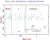 |
Figure 20:
Mass ratios of ELM WD. Vertical lines separate binaries which will, upon RLOF, exchange mass definitely stably (possible progenitors of AM CVn stars), WD for which stability of mass-exchange will depend on the efficiency of tidal interaction, and definitely unstable stars. The latter systems may be progenitors of SNe Ia, as discussed in Section 7.3.2. Courtesy T. Marsh [459]. |
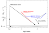 |
Figure 21:
Sketch of the period – mass transfer rate evolution of the binaries in the three proposed formation channels of AM CVn stars (the dashed line shows the detached phase of the white dwarf channel). For comparison, the evolutionary path of an ordinary hydrogen-rich CV or low-mass X-ray binary is shown. Image reproduced with permission from Figure 1 of [521], copyright by the authors. |
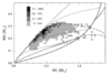 |
Figure 22:
Birthrates and stability limits for mass transfer between close WD binaries. The shaded areas show the birth probability of progenitors of AM CVn stars in double-degenerate channel scaled to the maximum birth rate per bin of  [518]. The upper dashed line corresponds to
the upper limit for stable mass transfer. The lower solid line is the lower limit for direct accretion.
The upper dash-dot line is the limit set by the Eddington luminosity for stable mass transfer at
a synchronization time limit [518]. The upper dashed line corresponds to
the upper limit for stable mass transfer. The lower solid line is the lower limit for direct accretion.
The upper dash-dot line is the limit set by the Eddington luminosity for stable mass transfer at
a synchronization time limit  . The lower dash-dot line is the limit set by the Eddington
luminosity for . The lower dash-dot line is the limit set by the Eddington
luminosity for  , and the lower broken line is the strict stability limit for the same. The
three dotted lines show how the strict stability limit is raised for shorter synchronization time-scales
ranging from 1000 yr (bottom), 10 yr (center), and 0.1 yr (top). Image reproduced with permission
from Figure 3 of [725], copyright by ASP. , and the lower broken line is the strict stability limit for the same. The
three dotted lines show how the strict stability limit is raised for shorter synchronization time-scales
ranging from 1000 yr (bottom), 10 yr (center), and 0.1 yr (top). Image reproduced with permission
from Figure 3 of [725], copyright by ASP. |
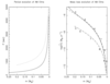 |
Figure 23:
Examples of the evolution of AM CVn systems. Left panel: The evolution of the orbital period as a function of the mass of the donor star. Right panel: The change of the mass transfer rate during the evolution. The solid and dashed lines are for zero-temperature white dwarf donor stars with initial mass  transferring matter to a primary with initial mass of 0.4 and transferring matter to a primary with initial mass of 0.4 and
 , respectively, assuming efficient coupling between the accretor spin and the orbital motion.
The dash-dotted and dotted lines are for a helium star donor, starting when the helium star becomes
semi-degenerate (with a mass of , respectively, assuming efficient coupling between the accretor spin and the orbital motion.
The dash-dotted and dotted lines are for a helium star donor, starting when the helium star becomes
semi-degenerate (with a mass of  ). Primaries are again ). Primaries are again  and and  . The numbers
along the lines indicate the logarithm of time in years since the beginning of mass transfer. Image
reproduced with permission from [512], copyright by ESO. . The numbers
along the lines indicate the logarithm of time in years since the beginning of mass transfer. Image
reproduced with permission from [512], copyright by ESO. |
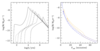 |
Figure 24:
Left panel: the  evolution of AM CVn systems with evolution of AM CVn systems with 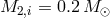 and and
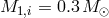 . Systems with donors having the degeneracy parameter . Systems with donors having the degeneracy parameter  = 3.5, 3.0,
2.5, 2.0, 1.5 and 1.1 are shown by the solid, dotted, short-dashed, dashed, shortdash-dotted and
dash-dotted lines, respectively. Right panel: the dependence of the = 3.5, 3.0,
2.5, 2.0, 1.5 and 1.1 are shown by the solid, dotted, short-dashed, dashed, shortdash-dotted and
dash-dotted lines, respectively. Right panel: the dependence of the  relation on the initial
binary parameters for pairs relation on the initial
binary parameters for pairs  , ,  (yellow dashed line), (yellow dashed line),
 , ,
 (yellow dot-dashed line), (yellow dot-dashed line),  , ,  (blue
dashed line), (blue
dashed line),  , ,  (blue dot-dashed line). Image
reproduced with permission from Figures 6 and 10 of [142], copyright by the authors. (blue dot-dashed line). Image
reproduced with permission from Figures 6 and 10 of [142], copyright by the authors. |
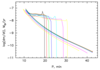 |
Figure 25:
Mass-loss rate vs. orbital period dependence for semidetached systems with He-star donors and WD accretors, having post-common envelope  to 130 min. Initial masses of
components are to 130 min. Initial masses of
components are  . He abundance in the cores of the donors at
RLOF ranges from 0.98 to 0.066 (left to right). Image from [870], copyright by the author. . He abundance in the cores of the donors at
RLOF ranges from 0.98 to 0.066 (left to right). Image from [870], copyright by the author. |
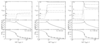 |
Figure 26:
An overview of the evolution and chemical abundances in the transferred matter for helium star donors in ultra-compact binaries. We show abundances (top), mass-transfer rate (middle) and donor mass (bottom) as a function of time since the start of the Roche lobe overflow. The binary period is indicated by the solid circles in the bottom panels for  = 15, 20, 25, 30, 35, and
40 min. The initial (post-common-envelope) orbital periods are indicated in the bottom panels. The
sequences differ by the amount of nuclear processing before RLOF. Image reproduced with permission
from Figure 4 of [521], copyright by the authors. = 15, 20, 25, 30, 35, and
40 min. The initial (post-common-envelope) orbital periods are indicated in the bottom panels. The
sequences differ by the amount of nuclear processing before RLOF. Image reproduced with permission
from Figure 4 of [521], copyright by the authors. |
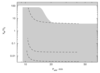 |
Figure 27:
Abundance ratios (by mass) N/C for He-WD (the solid line) and He-star donors (the shaded region with dashed lines) as a function of the orbital period. For the helium star donors we indicate the upper part of the full range of abundances which extends to 0. The dashed lines are examples of tracks shown in detail in Figure 26. The helium white dwarfs are descendants of 1, 1.5 and  stars (top to bottom). Image reproduced with permission from Figure 11 of [521],
copyright by the authors. stars (top to bottom). Image reproduced with permission from Figure 11 of [521],
copyright by the authors. |
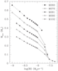 |
Figure 28:
Accreted mass as a function of the accretion rate for models experiencing a dynamical He-flash. The lines refer to WD with different initial masses — 0.6, 0.7, 0.81, 0.92, 1.02  .
Piersanti, Tornambé and Yungelson in prep. .
Piersanti, Tornambé and Yungelson in prep. |
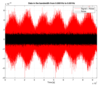 |
Figure 29:
Simulated time-series of the DD Galactic foreground signal of 3 years of data. “Noise” is the instrumental LISA noise. Based on computations in [519]. Image reproduced with permission from [170], copyright by ASP. |
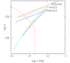 |
Figure 30:
Dependence of the dimensionless strain amplitude for a WD + WD detached system with initial masses of the components of  (red line), a WD + WD system with (red line), a WD + WD system with
 (blue line) and a NS + WD system with (blue line) and a NS + WD system with  (green line). All
systems have an initial separation of components (green line). All
systems have an initial separation of components  and are assumed to be at a distance of
1 Kpc (i.e., the actual strength of the signal has to be scaled with factor and are assumed to be at a distance of
1 Kpc (i.e., the actual strength of the signal has to be scaled with factor  , with , with  in Kpc).
For the DD system, the line shows an evolution into contact, while for the other two systems the
upper branches show pre-contact evolution and lower branches – a post-contact evolution with mass
exchange. The total time-span of evolution covered by the tracks is 13.5 Gyr. Red dots mark the
positions of systems with components’ mass ratio in Kpc).
For the DD system, the line shows an evolution into contact, while for the other two systems the
upper branches show pre-contact evolution and lower branches – a post-contact evolution with mass
exchange. The total time-span of evolution covered by the tracks is 13.5 Gyr. Red dots mark the
positions of systems with components’ mass ratio  , below which the conventional picture
of evolution with a mass exchange may be not valid. The red dashed line marks the position of the
confusion limit as determined in [519]. , below which the conventional picture
of evolution with a mass exchange may be not valid. The red dashed line marks the position of the
confusion limit as determined in [519]. |
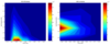 |
Figure 31:
The distribution of Galactic detached WD + WD binaries and interacting WD (AM CVn stars) as a function of the gravitational wave frequency and chirp mass. From [170], based on computations in [519]. |
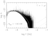 |
Figure 32:
GWR foreground produced by detached and semidetached WD binaries as it was expected to be detected by LISA. The assumed integration time is 1 yr. The ‘noisy’ black line gives the total power spectrum, the white line shows the average. The dashed lines show the expected LISA sensitivity for a  of 1 and 5 [408]. Semidetached WD binaries contribute to the peak between of 1 and 5 [408]. Semidetached WD binaries contribute to the peak between
 and and  . Image reproduced with permission from [518], copyright by ESO. . Image reproduced with permission from [518], copyright by ESO. |
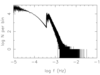 |
Figure 33:
The number of systems per bin on a logarithmic scale. Semidetached WD binaries contribute to the peak between  and and  . Image reproduced with permission
from [518], copyright by ESO. . Image reproduced with permission
from [518], copyright by ESO. |
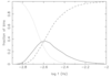 |
Figure 34:
Fraction of bins that contain exactly one system (solid line), empty bins (dashed line), and bins that contain more than one system (dotted line) as a function of the signal frequency. From [518], copyright by ESO. |
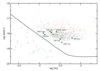 |
Figure 35:
Strain amplitude spectral density (in Hz–1/2) versus frequency for the verification binaries and the brightest binaries in the simulated Galactic population of ultra-compact binaries [519]. The solid line shows the sensitivity of eLISA. The assumed integration time is 2 yrs. 100 simulated binaries with the largest strain amplitude are shown as red squares. Observed ultra-compact binaries are shown as blue squares, while the subsample of them that can serve as verification binaries is marked as green squares. Image reproduced with permission from [11], copyright by the authors. |
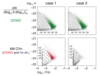 |
Figure 36:
The number density as a function of GW-strain amplitude  and frequency and frequency  for
close detached WD (top) and AM CVn stars (bottom) in Case 1 and Case 2. Green dots denote
individually-detected WD binary systems (for one year of observation with the 5-Mkm detector); red
dots – AM CVn systems from the WD binary channel and blue dots – AM CVn systems from the
He star channel. Image reproduced with permission from [531], copyright by AAS. for
close detached WD (top) and AM CVn stars (bottom) in Case 1 and Case 2. Green dots denote
individually-detected WD binary systems (for one year of observation with the 5-Mkm detector); red
dots – AM CVn systems from the WD binary channel and blue dots – AM CVn systems from the
He star channel. Image reproduced with permission from [531], copyright by AAS. |
 |
Figure 37:
The frequency-space density and GW foreground of DD and AM CVn systems for two scenarios. In each subplot, the bottom panel shows the power spectral density of the unsubtracted (blue) and partially subtracted (red) foreground, compared to instrumental noise (black). The open white circles indicate the frequency and amplitude of the “verification binaries”. The green dots show the individually-detectable DD systems; the red dots show the detectable AM CVn systems formed from DD progenitors and the blue dots show the detectable AM CVn systems that arise from the He-star–WD channel. The top panel shows histograms of the detected sources in the frequency space. Image reproduced with permission from [531], copyright by AAS. |
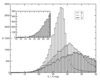 |
Figure 38:
The histogram of apparent magnitudes of the WD binaries that are estimated to be individually detected by LISA. The black-and-white line shows the distribution in the  -band, the
black line the distribution in the -band, the
black line the distribution in the  -band and the grey histogram the distribution in the -band and the grey histogram the distribution in the  -band.
Galactic absorption is taken into account. The insert shows the bright-end tail of the -band.
Galactic absorption is taken into account. The insert shows the bright-end tail of the  -band
distribution. Image reproduced with permission from [509], copyright by IOP. -band
distribution. Image reproduced with permission from [509], copyright by IOP. |
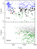 |
Figure 39:
Distribution of short period AM CVn-type systems detectable in soft X-ray and as optical sources as a function of the orbital period and distance. Top panel: systems detectable in X-ray only (blue pluses), direct impact systems observable in X-ray and  -band (red filled circles),
systems detectable in X-ray with an optically visible donor (green squares), and systems detectable in
X-ray and with an optically visible disc (large filled triangles). Bottom panel: direct impact systems
(red open circles), systems with a visible donor (green squares), and systems with a visible accretion
disc (small open triangles). The sample is limited by -band (red filled circles),
systems detectable in X-ray with an optically visible donor (green squares), and systems detectable in
X-ray and with an optically visible disc (large filled triangles). Bottom panel: direct impact systems
(red open circles), systems with a visible donor (green squares), and systems with a visible accretion
disc (small open triangles). The sample is limited by  . Image reproduced with permission
from Figure 1 of [519], copyright by the authors. . Image reproduced with permission
from Figure 1 of [519], copyright by the authors. |
Konstantin A. Postnov and Lev R. Yungelson, "The Evolution of Compact Binary Star Systems",
Living Rev. Relativity, 17 (2014), 3, doi:10.12942/lrr-2014-3, URL (accessed <date>): http://www.livingreviews.org/lrr-2014-3. This work is licensed under a Creative Commons License.
© The author(s), except where otherwise noted.
This work is licensed under a Creative Commons License.
© The author(s), except where otherwise noted.
Living Rev. Relativity, 17 (2014), 3, doi:10.12942/lrr-2014-3, URL (accessed <date>): http://www.livingreviews.org/lrr-2014-3.
This work is licensed under a Creative Commons License.
© The author(s), except where otherwise noted.