9 Gravitational Waves from Compact Binaries
We pointed out that the 3.5PN equations of motion, Eqs. (203) or (219*) – (220), are merely 1PN as regards the radiative aspects of the problem, because the radiation reaction force starts at the 2.5PN order. A solution would be to extend the precision of the equations of motion so as to include the full relative 3PN or 3.5PN precision into the radiation reaction force, but the equations of motion up to the 5.5PN or 6PN order are beyond the present state-of-the-art. The much better alternative solution is to apply the wave-generation formalism described in Part A, and to determine by its means the work done by the radiation reaction force directly as a total energy flux at future null infinity.62 In this approach, we replace the knowledge of the higher-order radiation reaction force by the computation of the total flux , and we apply the energy balance equation
Therefore, the result (232) that we found for the 3.5PN binary’s center-of-mass energy
, and we apply the energy balance equation
Therefore, the result (232) that we found for the 3.5PN binary’s center-of-mass energy 
 constitutes only
“half” of the solution of the problem. The second “half” consists of finding the rate of decrease
constitutes only
“half” of the solution of the problem. The second “half” consists of finding the rate of decrease  ,
which by the balance equation is nothing but the total gravitational-wave flux
,
which by the balance equation is nothing but the total gravitational-wave flux  at the relative 3.5PN
order beyond the Einstein quadrupole formula (4*).
at the relative 3.5PN
order beyond the Einstein quadrupole formula (4*).
Because the orbit of inspiralling binaries is circular, the energy balance equation is sufficient, and there
is no need to invoke the angular momentum balance equation for computing the evolution of the orbital
period  and eccentricity
  , see Eqs. (9) – (13*) in the case of the binary pulsar. Furthermore the time
average over one orbital period as in Eqs. (9) is here irrelevant, and the energy and angular
momentum fluxes are related by
, see Eqs. (9) – (13*) in the case of the binary pulsar. Furthermore the time
average over one orbital period as in Eqs. (9) is here irrelevant, and the energy and angular
momentum fluxes are related by  . This all sounds good, but it is important to remind
that we shall use the balance equation (295*) at the very high 3.5PN order, and that at such
order one is missing a complete proof of it (following from first principles in general relativity).
Nevertheless, in addition to its physically obvious character, Eq. (295*) has been verified by
radiation-reaction calculations, in the cases of point-particle binaries [258, 259] and extended
post-Newtonian fluids [43, 47], at the 1PN order and even at 1.5PN, the latter order being especially
important because of the first appearance of wave tails; see Section 5.4. One should also quote here
Refs. [260, 336, 278, 322, 254] for the 3.5PN terms in the binary’s equations of motion, fully consistent
with the balance equations.
. This all sounds good, but it is important to remind
that we shall use the balance equation (295*) at the very high 3.5PN order, and that at such
order one is missing a complete proof of it (following from first principles in general relativity).
Nevertheless, in addition to its physically obvious character, Eq. (295*) has been verified by
radiation-reaction calculations, in the cases of point-particle binaries [258, 259] and extended
post-Newtonian fluids [43, 47], at the 1PN order and even at 1.5PN, the latter order being especially
important because of the first appearance of wave tails; see Section 5.4. One should also quote here
Refs. [260, 336, 278, 322, 254] for the 3.5PN terms in the binary’s equations of motion, fully consistent
with the balance equations.
Obtaining the energy flux  can be divided into two equally important steps: Computing the source
multipole moments
can be divided into two equally important steps: Computing the source
multipole moments  and
and  of the compact binary system with due account of a self-field
regularization; and controlling the tails and related non-linear effects occurring in the relation between the
binary’s source moments and the radiative ones
of the compact binary system with due account of a self-field
regularization; and controlling the tails and related non-linear effects occurring in the relation between the
binary’s source moments and the radiative ones  and
and  observed at future null infinity (cf. the
general formalism of Part A).
observed at future null infinity (cf. the
general formalism of Part A).
9.1 The binary’s multipole moments
The general expressions of the source multipole moments given by Theorem 6, Eqs. (123), are
worked out explicitly for general fluid systems at the 3.5PN order. For this computation one
uses the formula (126*), and we insert the 3.5PN metric coefficients (in harmonic coordinates)
expressed in Eqs. (144) by means of the retarded-type elementary potentials (146) – (148).
Then we specialize each of the (quite numerous) terms to the case of point-particle binaries by
inserting, for the matter stress-energy tensor  , the standard expression made out of Dirac
delta-functions. In Section 11 we shall consider spinning point particle binaries, and in that case the
stress-energy tensor is given by Eq. (378*). The infinite self-field of point-particles is removed
by means of the Hadamard regularization; and, as we discussed in Section 6.4, dimensional
regularization is used to fix the values of a few ambiguity parameters. This computation has been
performed in Ref. [86*] at the 1PN order, and in [64] at the 2PN order; we report below the most
accurate 3PN results obtained in Refs. [81*, 80, 62, 63] for the flux and [11*, 74*, 197*] for the
waveform.
, the standard expression made out of Dirac
delta-functions. In Section 11 we shall consider spinning point particle binaries, and in that case the
stress-energy tensor is given by Eq. (378*). The infinite self-field of point-particles is removed
by means of the Hadamard regularization; and, as we discussed in Section 6.4, dimensional
regularization is used to fix the values of a few ambiguity parameters. This computation has been
performed in Ref. [86*] at the 1PN order, and in [64] at the 2PN order; we report below the most
accurate 3PN results obtained in Refs. [81*, 80, 62, 63] for the flux and [11*, 74*, 197*] for the
waveform.
A difficult part of the analysis is to find the closed-form expressions, fully explicit in terms of the particle’s positions and velocities, of many non-linear integrals. Let us give a few examples of the type of technical formulas that are employed in this calculation. Typically we have to compute some integrals like
where
 and
and  . When
  and
and  , this integral is perfectly
well-defined, since the finite part
, this integral is perfectly
well-defined, since the finite part  deals with the IR regularization of the bound at infinity. When
 or
or  , we cure the UV divergencies by means of the Hadamard partie finie defined by
Eq. (162*); so a partie finie prescription
, we cure the UV divergencies by means of the Hadamard partie finie defined by
Eq. (162*); so a partie finie prescription  is implicit in Eq. (296*). An example of closed-form formula we
get is
where we pose
is implicit in Eq. (296*). An example of closed-form formula we
get is
where we pose 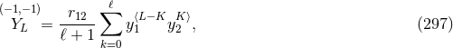
 and
and 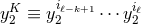 , the brackets surrounding indices denoting
the STF projection. Another example, in which the
, the brackets surrounding indices denoting
the STF projection. Another example, in which the  regularization is crucial, is (in the quadrupole
case
regularization is crucial, is (in the quadrupole
case  )
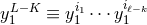
where the IR scale
)
where the IR scale ![(− 2,−1) [16 (r ) 188 ] [ 8 ( r ) 4 ] [2 ( r ) 2] Yij = y⟨1ij⟩ ---ln --12 − ---- + y⟨1i yj2⟩ --ln -12- − ---- + y⟨2ij⟩ --ln -12 − --- ,(298 ) 15 r0 225 15 r0 225 5 r0 25](article2234x.gif)
 is defined in Eq. (42*). Still another example, which necessitates both the
  and
a UV partie finie regularization at the point 1, is
where
and
a UV partie finie regularization at the point 1, is
where ![(−3,0) [ ( s ) 16] Yij = 2 ln -1 + --- y⟨1ij⟩, (299 ) r0 15](article2237x.gif)
 is the Hadamard-regularization constant introduced in Eq. (162*).
The most important input for the computation of the waveform and flux is the mass quadrupole
moment  , since this moment necessitates the full post-Newtonian precision. Here we give the mass
quadrupole moment complete to order 3.5PN, for non-spinning compact binaries on circular orbits, as
, since this moment necessitates the full post-Newtonian precision. Here we give the mass
quadrupole moment complete to order 3.5PN, for non-spinning compact binaries on circular orbits, as

 and
and  are the orbital separation and relative velocity. The
third term with coefficient
are the orbital separation and relative velocity. The
third term with coefficient  is a radiation-reaction term, which will affect the waveform at
orders 2.5PN and 3.5PN; however it does not contribute to the energy flux for circular orbits.
The two conservative coefficients are
is a radiation-reaction term, which will affect the waveform at
orders 2.5PN and 3.5PN; however it does not contribute to the energy flux for circular orbits.
The two conservative coefficients are  and
and  . All those coefficients are [81*, 74*, 197*]
These expressions are valid in harmonic coordinates via the post-Newtonian parameter  defined in Eq. (225*). As we see, there are two types of logarithms at 3PN order in the quadrupole moment:
One type involves the UV length scale
defined in Eq. (225*). As we see, there are two types of logarithms at 3PN order in the quadrupole moment:
One type involves the UV length scale  related by Eq. (221*) to the two gauge constants
  and
and  present in the 3PN equations of motion; the other type contains the IR length scale
  coming from the
general formalism of Part A – indeed, recall that there is a
coming from the
general formalism of Part A – indeed, recall that there is a  operator in front of the source multipole
moments in Theorem 6. As we know, the UV scale
operator in front of the source multipole
moments in Theorem 6. As we know, the UV scale  is specific to the standard harmonic
(SH) coordinate system and is pure gauge (see Section 7.3): It will disappear from our physical
results at the end. On the other hand, we have proved that the multipole expansion outside a
general post-Newtonian source is actually free of
is specific to the standard harmonic
(SH) coordinate system and is pure gauge (see Section 7.3): It will disappear from our physical
results at the end. On the other hand, we have proved that the multipole expansion outside a
general post-Newtonian source is actually free of  , since the
  ’s present in the two terms
of Eq. (105*) cancel out. Indeed we have already found in Eqs. (93*) – (94*) that the constant
’s present in the two terms
of Eq. (105*) cancel out. Indeed we have already found in Eqs. (93*) – (94*) that the constant
 present in
  is compensated by the same constant coming from the non-linear wave
“tails of tails” in the radiative moment
is compensated by the same constant coming from the non-linear wave
“tails of tails” in the radiative moment  . For a while, the expressions (301) contained
the ambiguity parameters
. For a while, the expressions (301) contained
the ambiguity parameters  ,
,  and
and  , which have now been replaced by their correct
values (173).
, which have now been replaced by their correct
values (173).
Besides the 3.5PN mass quadrupole (300*) – (301), we need also (for the 3PN waveform) the mass
octupole moment  and current quadrupole moment
  , both of them at the 2.5PN order; these are
given for circular orbits by [81*, 74*]
, both of them at the 2.5PN order; these are
given for circular orbits by [81*, 74*]
The list of required source moments for the 3PN waveform continues with the 2PN mass
 -pole and current
  -pole (octupole) moments, and so on. Here we give the most updated
moments:63
-pole (octupole) moments, and so on. Here we give the most updated
moments:63
All the other higher-order moments are required at the Newtonian order, at which they are trivial to
compute with result ( )
)
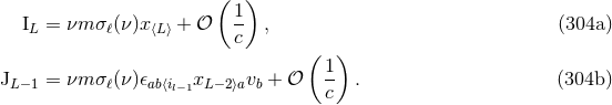
Here we introduce the useful notation 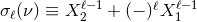 , where
  and
and  are
such that
are
such that  ,
, 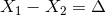 and
and  . More explicit expressions are (
 ):
):
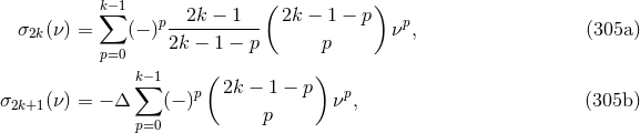
where  is the usual binomial coefficient.
9.2 Gravitational wave energy flux
The results (300*) – (304) permit the control of the instantaneous part of the total energy flux, by which we
mean that part of the flux which is generated solely by the source multipole moments, i.e., not counting the
hereditary tail and related integrals. The instantaneous flux  is defined by the replacement into the
general expression of
is defined by the replacement into the
general expression of  given by Eq. (68a) of all the radiative moments
  and
and  by the
corresponding
by the
corresponding  -th time derivatives of the source moments
  and
and  . Up to the 3.5PN order we
have
. Up to the 3.5PN order we
have
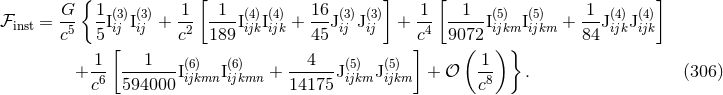
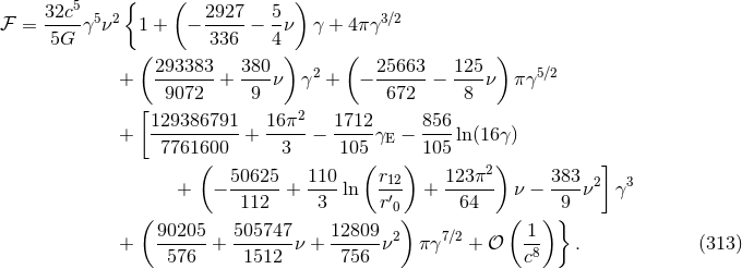
in which we insert the explicit expressions (300*) – (304) for the moments. The time derivatives of these source moments are computed by means of the circular-orbit equations of motion given by Eq. (226*) together with (228). The net result is
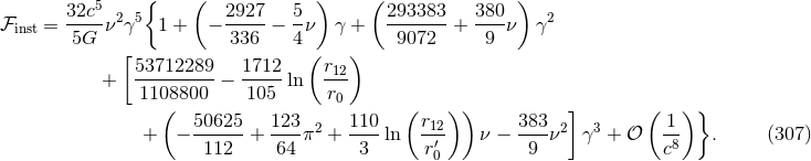
The Newtonian approximation agrees with the prediction of the Einstein quadrupole formula (4*), as reduced for quasi-circular binary orbits by Landau & Lifshitz [285]. At the 3PN order in Eq. (307), there was some Hadamard regularization ambiguity parameters which have been replaced by their values computed with dimensional regularization.
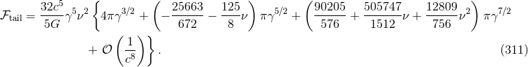
To the instantaneous part of the flux, we must add the contribution of non-linear multipole interactions contained in the relationship between the source and radiative moments. The needed material has already been provided in Sections 3.3. Similar to the decomposition of the radiative quadrupole moment in Eq. (88*), we can split the energy flux into the different terms
where
 has just been obtained in Eq. (307);
  is made of the quadratic multipolar tail integrals
in Eqs. (90) and (95);
is made of the quadratic multipolar tail integrals
in Eqs. (90) and (95);  involves the square of the quadrupole tail in Eq. (90) and the quadrupole
tail of tail given in Eq. (91).
involves the square of the quadrupole tail in Eq. (90) and the quadrupole
tail of tail given in Eq. (91).
We shall see that the tails play a crucial role in the predicted signal of compact binaries. It is quite remarkable that so small an effect as a “tail of tail” should be relevant to the data analysis of the current generation of gravitational wave detectors. By contrast, the non-linear memory effects, given by the integrals inside the 2.5PN and 3.5PN terms in Eq. (92), do not contribute to the gravitational-wave energy flux before the 4PN order in the case of circular-orbit binaries. Indeed the memory integrals are actually “instantaneous” in the flux, and a simple general argument based on dimensional analysis shows that instantaneous terms cannot contribute to the energy flux for circular orbits.64 Therefore the memory effect has rather poor observational consequences for future detections of inspiralling compact binaries.
Let us also recall that following the general formalism of Part A, the mass  which appears
in front of the tail integrals of Sections 3.2 and 3.3 represents the binary’s mass monopole
which appears
in front of the tail integrals of Sections 3.2 and 3.3 represents the binary’s mass monopole
 or ADM mass. In a realistic model where the binary system has been formed as a close
compact binary at a finite instant in the past, this mass is equal to the sum of the rest masses
or ADM mass. In a realistic model where the binary system has been formed as a close
compact binary at a finite instant in the past, this mass is equal to the sum of the rest masses
 , plus the total binary’s mass-energy
  given for instance by Eq. (229). At
3.5PN order we need 2PN corrections in the tails and therefore 2PN also in the mass
given for instance by Eq. (229). At
3.5PN order we need 2PN corrections in the tails and therefore 2PN also in the mass  , thus
![[ ( )] ν- ν- 2 -1 M = m 1 − 2 γ + 8 (7 − ν)γ + 𝒪 c6 . (309 )](article2301x.gif)
 corresponds to 1PN order in
  .
.
We give the two basic technical formulas needed when carrying out the reduction of the tail and tail-of-tail integrals to circular orbits (see e.g., [230]):
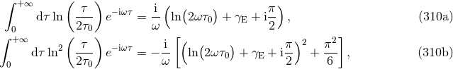
where  is a strictly positive frequency (a multiple of the orbital frequency
  ), where
 and
and  is the Euler constant.
Notice the important point that the tail (and tail-of-tail) integrals can be evaluated, thanks to these
formulas, for a fixed (i.e., non-decaying) circular orbit. Indeed it can be shown [60, 87*] that the “remote-past”
contribution to the tail integrals is negligible; the errors due to the fact that the orbit has actually evolved
in the past, and spiraled in by emission of gravitational radiation, are of the order of the radiation-reaction scale
 ,65
and do not affect the signal before the 4PN order. We then find, for the quadratic tails stricto sensu, the
1.5PN, 2.5PN and 3.5PN contributions
,65
and do not affect the signal before the 4PN order. We then find, for the quadratic tails stricto sensu, the
1.5PN, 2.5PN and 3.5PN contributions
For the sum of squared tails and cubic tails of tails at 3PN, we get
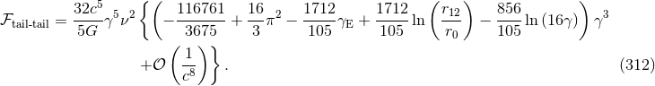
By comparing Eqs. (307) and (312) we observe that the constants  cleanly cancel out. Adding
together these contributions we obtain
cleanly cancel out. Adding
together these contributions we obtain
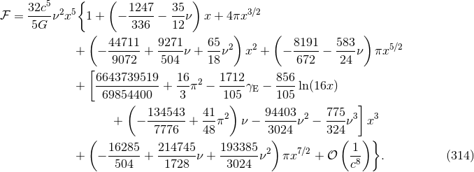
The gauge constant  has not yet disappeared because the post-Newtonian expansion is still parametrized
by
has not yet disappeared because the post-Newtonian expansion is still parametrized
by  instead of the frequency-related parameter
  defined by Eq. (230*) – just as for
  when it was
given by Eq. (229). After substituting the expression
when it was
given by Eq. (229). After substituting the expression  given by Eq. (231), we find that
  does
cancel as well. Because the relation
does
cancel as well. Because the relation  is issued from the equations of motion, the latter cancellation
represents an interesting test of the consistency of the two computations, in harmonic coordinates, of the
3PN multipole moments and the 3PN equations of motion. At long last we obtain our end
result:66
is issued from the equations of motion, the latter cancellation
represents an interesting test of the consistency of the two computations, in harmonic coordinates, of the
3PN multipole moments and the 3PN equations of motion. At long last we obtain our end
result:66
In the test-mass limit  for one of the bodies, we recover exactly the result following from linear
black-hole perturbations obtained by Tagoshi & Sasaki [395] (see also [393, 397]). In particular, the
rational fraction
for one of the bodies, we recover exactly the result following from linear
black-hole perturbations obtained by Tagoshi & Sasaki [395] (see also [393, 397]). In particular, the
rational fraction  comes out exactly the same as in black-hole perturbations. On the other hand,
the ambiguity parameters discussed in Section 6.2 were part of the rational fraction
comes out exactly the same as in black-hole perturbations. On the other hand,
the ambiguity parameters discussed in Section 6.2 were part of the rational fraction  , belonging to
the coefficient of the term at 3PN order proportional to
, belonging to
the coefficient of the term at 3PN order proportional to  (hence this coefficient cannot be computed by
linear black-hole perturbations).
(hence this coefficient cannot be computed by
linear black-hole perturbations).
The effects due to the spins of the two black holes arise at the 1.5PN order for the spin-orbit (SO) coupling, and at the 2PN order for the spin-spin (SS) coupling, for maximally rotating black holes. Spin effects will be discussed in Section 11. On the other hand, the terms due to the radiating energy flowing into the black-hole horizons and absorbed rather than escaping to infinity, have to be added to the standard post-Newtonian calculation based on point particles as presented here; such terms arise at the 4PN order for Schwarzschild black holes [349*] and at 2.5PN order for Kerr black holes [392*].
9.3 Orbital phase evolution
We shall now deduce the laws of variation with time of the orbital frequency and phase of an inspiralling
compact binary from the energy balance equation (295*). The center-of-mass energy  is given by
Eq. (232) and the total flux
is given by
Eq. (232) and the total flux  by Eq. (314). For convenience we adopt the dimensionless time
variable67
by Eq. (314). For convenience we adopt the dimensionless time
variable67

 denotes the instant of coalescence, at which the frequency formally tends to infinity, although
evidently, the post-Newtonian method breaks down well before this point. We transform the balance
equation into an ordinary differential equation for the parameter
denotes the instant of coalescence, at which the frequency formally tends to infinity, although
evidently, the post-Newtonian method breaks down well before this point. We transform the balance
equation into an ordinary differential equation for the parameter  , which is immediately integrated with
the result
, which is immediately integrated with
the result
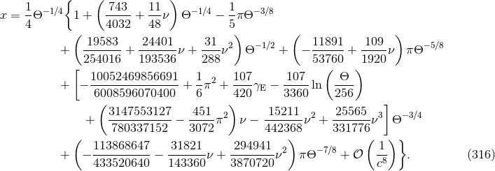
The orbital phase is defined as the angle  , oriented in the sense of the motion, between the separation of
the two bodies and the direction of the ascending node (called
, oriented in the sense of the motion, between the separation of
the two bodies and the direction of the ascending node (called  in Section 9.4) within the plane of the
sky. We have
in Section 9.4) within the plane of the
sky. We have  , which translates, with our notation, into
 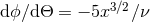 , from which we
determine68
, from which we
determine68
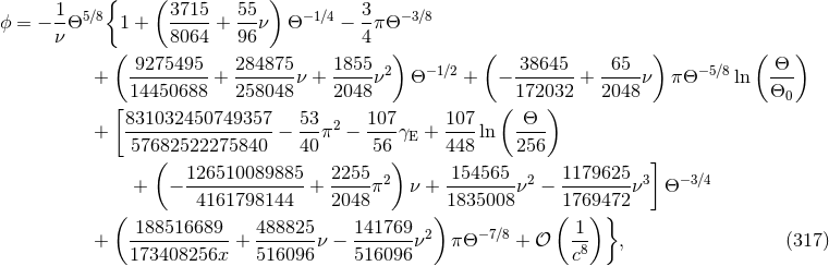
where  is a constant of integration that can be fixed by the initial conditions when the wave
frequency enters the detector. Finally we want also to dispose of the important expression of the phase in
terms of the frequency
is a constant of integration that can be fixed by the initial conditions when the wave
frequency enters the detector. Finally we want also to dispose of the important expression of the phase in
terms of the frequency  . For this we get
where  is another constant of integration. With the formula (318) the orbital phase is complete up
to the 3.5PN order for non-spinning compact binaries. Note that the contributions of the quadrupole
moments of compact objects which are induced by tidal effects, are expected from Eq. (16*) to come into
play only at the 5PN order.
is another constant of integration. With the formula (318) the orbital phase is complete up
to the 3.5PN order for non-spinning compact binaries. Note that the contributions of the quadrupole
moments of compact objects which are induced by tidal effects, are expected from Eq. (16*) to come into
play only at the 5PN order.
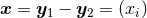
As a rough estimate of the relative importance of the various post-Newtonian terms, we give in Table 3
their contributions to the accumulated number of gravitational-wave cycles  in the bandwidth of
ground-based detectors. Note that such an estimate is only indicative, because a full treatment would
require the knowledge of the detector’s power spectral density of noise, and a complete simulation of the
parameter estimation using matched filtering techniques [138*, 350, 284]. We define
in the bandwidth of
ground-based detectors. Note that such an estimate is only indicative, because a full treatment would
require the knowledge of the detector’s power spectral density of noise, and a complete simulation of the
parameter estimation using matched filtering techniques [138*, 350, 284]. We define  as
as

 of
ground-based detectors; the terminal frequency is assumed for simplicity to be given by the Schwarzschild
innermost stable circular orbit:
of
ground-based detectors; the terminal frequency is assumed for simplicity to be given by the Schwarzschild
innermost stable circular orbit:  . Here we denote by
  the signal
frequency of the dominant harmonics at twice the orbital frequency. As we see in Table 3, with the 3PN or
3.5PN approximations we reach an acceptable accuracy level of a few cycles say, that roughly corresponds
to the demand made by data-analysists in the case of neutron-star binaries [139, 137, 138*, 346, 105*, 106*].
Indeed, the above estimation suggests that the neglected 4PN terms will yield some systematic
errors that are, at most, of the same order of magnitude, i.e., a few cycles, and perhaps much
less.
the signal
frequency of the dominant harmonics at twice the orbital frequency. As we see in Table 3, with the 3PN or
3.5PN approximations we reach an acceptable accuracy level of a few cycles say, that roughly corresponds
to the demand made by data-analysists in the case of neutron-star binaries [139, 137, 138*, 346, 105*, 106*].
Indeed, the above estimation suggests that the neglected 4PN terms will yield some systematic
errors that are, at most, of the same order of magnitude, i.e., a few cycles, and perhaps much
less.
 for compact binaries detectable in the bandwidth of LIGO-VIRGO detectors. The entry
frequency is
for compact binaries detectable in the bandwidth of LIGO-VIRGO detectors. The entry
frequency is  and the terminal frequency is
  . The main origin of
the approximation (instantaneous vs. tail) is indicated. See also Table 4 in Section 11 below for the
contributions of spin-orbit effects.
. The main origin of
the approximation (instantaneous vs. tail) is indicated. See also Table 4 in Section 11 below for the
contributions of spin-orbit effects.| PN order |  |
 |
 |
|
| N | (inst) | 15952.6 | 3558.9 | 598.8 |
| 1PN | (inst) | 439.5 | 212.4 | 59.1 |
| 1.5PN | (leading tail) | –210.3 | –180.9 | –51.2 |
| 2PN | (inst) | 9.9 | 9.8 | 4.0 |
| 2.5PN | (1PN tail) | –11.7 | –20.0 | –7.1 |
| 3PN | (inst + tail-of-tail) | 2.6 | 2.3 | 2.2 |
| 3.5PN | (2PN tail) | –0.9 | –1.8 | –0.8 |
9.4 Polarization waveforms for data analysis
The theoretical templates of the compact binary inspiral follow from insertion of the previous solutions for
the 3.5PN-accurate orbital frequency and phase into the binary’s two polarization waveforms  and
and
 defined with respect to a choice of two polarization vectors
  and
and  orthogonal to
the direction
orthogonal to
the direction  of the observer; see Eqs. (69).
Our convention for the two polarization vectors is that they form with  a right-handed triad, and
that
a right-handed triad, and
that  and
and  lie along the major and minor axis, respectively, of the projection onto the plane of the
sky of the circular orbit. This means that
lie along the major and minor axis, respectively, of the projection onto the plane of the
sky of the circular orbit. This means that  is oriented toward the orbit’s ascending node – namely the
point
is oriented toward the orbit’s ascending node – namely the
point  at which the orbit intersects the plane of the sky and the bodies are moving toward the observer
located in the direction
at which the orbit intersects the plane of the sky and the bodies are moving toward the observer
located in the direction  . The ascending node is also chosen for the origin of the orbital
phase
. The ascending node is also chosen for the origin of the orbital
phase  . We denote by
  the inclination angle between the direction of the detector
  as
seen from the binary’s center-of-mass, and the normal to the orbital plane (we always suppose
that the normal is right-handed with respect to the sense of motion, so that
as
seen from the binary’s center-of-mass, and the normal to the orbital plane (we always suppose
that the normal is right-handed with respect to the sense of motion, so that  ).
We use the shorthands
).
We use the shorthands  and
and  for the cosine and sine of the inclination
angle.
for the cosine and sine of the inclination
angle.
We shall include in  and
and  all the harmonics, besides the dominant one at twice the orbital
frequency, consistent with the 3PN approximation [82, 11*, 74*]. In Section 9.5 we shall give all
the modes
all the harmonics, besides the dominant one at twice the orbital
frequency, consistent with the 3PN approximation [82, 11*, 74*]. In Section 9.5 we shall give all
the modes  in a spherical-harmonic decomposition of the waveform, and shall extend
the dominant quadrupole mode
in a spherical-harmonic decomposition of the waveform, and shall extend
the dominant quadrupole mode  at 3.5PN order [197*]. The post-Newtonian terms are
ordered by means of the frequency-related variable
at 3.5PN order [197*]. The post-Newtonian terms are
ordered by means of the frequency-related variable  ; to ease the notation we pose

 starting at 3PN order; see
Eq. (127*). They depend on the binary’s phase
starting at 3PN order; see
Eq. (127*). They depend on the binary’s phase  , explicitly given at 3.5PN order by Eq. (318), through
the very useful auxiliary phase variable
, explicitly given at 3.5PN order by Eq. (318), through
the very useful auxiliary phase variable  that is “distorted by tails” [87*, 11*] and reads
Here
that is “distorted by tails” [87*, 11*] and reads
Here 
 denotes the binary’s ADM mass and it is very important to include all its relevant
post-Newtonian contributions as given by Eq. (309*). The constant frequency
denotes the binary’s ADM mass and it is very important to include all its relevant
post-Newtonian contributions as given by Eq. (309*). The constant frequency  can be chosen
at will, for instance to be the entry frequency of some detector. For the plus polarization we
have69
can be chosen
at will, for instance to be the entry frequency of some detector. For the plus polarization we
have69
For the cross polarizations we obtain
Notice the non-linear memory zero-frequency (DC) term present in the Newtonian plus polarization
 ; see Refs. [427, 11, 189*] for the computation of this term. Notice also that there is another DC term
in the 2.5PN cross polarization
; see Refs. [427, 11, 189*] for the computation of this term. Notice also that there is another DC term
in the 2.5PN cross polarization  , first term in Eq. (323f).
The practical implementation of the theoretical templates in the data analysis of detectors follows from
the standard matched filtering technique. The raw output of the detector  consists of the
superposition of the real gravitational wave signal
consists of the
superposition of the real gravitational wave signal  and of noise
  . The noise is assumed to be
a stationary Gaussian random variable, with zero expectation value, and with (supposedly known)
frequency-dependent power spectral density
. The noise is assumed to be
a stationary Gaussian random variable, with zero expectation value, and with (supposedly known)
frequency-dependent power spectral density  . The experimenters construct the correlation between
 and a filter
  , i.e.,

 by the square root of its variance, or correlation noise. The expectation value of this ratio
defines the filtered signal-to-noise ratio (SNR). Looking for the useful signal
by the square root of its variance, or correlation noise. The expectation value of this ratio
defines the filtered signal-to-noise ratio (SNR). Looking for the useful signal  in the detector’s
output
in the detector’s
output  , the data analysists adopt for the filter
where
, the data analysists adopt for the filter
where 
 and
and  are the Fourier transforms of
  and of the theoretically computed template
 . By the matched filtering theorem, the filter (325*) maximizes the SNR if
  . The
maximum SNR is then the best achievable with a linear filter. In practice, because of systematic errors in
the theoretical modelling, the template
. The
maximum SNR is then the best achievable with a linear filter. In practice, because of systematic errors in
the theoretical modelling, the template  will not exactly match the real signal
  ;
however if the template is to constitute a realistic representation of nature the errors will be
small. This is of course the motivation for computing high order post-Newtonian templates, in
order to reduce as much as possible the systematic errors due to the unknown post-Newtonian
remainder.
;
however if the template is to constitute a realistic representation of nature the errors will be
small. This is of course the motivation for computing high order post-Newtonian templates, in
order to reduce as much as possible the systematic errors due to the unknown post-Newtonian
remainder.
To conclude, the use of theoretical templates based on the preceding 3PN/3.5PN waveforms, and having their frequency evolution built in via the 3.5PN phase evolution (318) [recall also the “tail-distorted” phase variable (321*)], should yield some accurate detection and measurement of the binary signals, whose inspiral phase takes place in the detector’s bandwidth [105, 106, 159, 156, 3, 18, 111]. Interestingly, it should also permit some new tests of general relativity, because we have the possibility of checking that the observed signals do obey each of the terms of the phasing formula (318) – particularly interesting are those terms associated with non-linear tails – exactly as they are predicted by Einstein’s theory [84, 85, 15, 14]. Indeed, we don’t know of any other physical systems for which it would be possible to perform such tests.
9.5 Spherical harmonic modes for numerical relativity
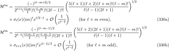
The spin-weighted spherical harmonic modes of the polarization waveforms have been defined in Eq. (71*).
They can be evaluated either from applying the angular integration formula (72*), or alternatively from
using the relations (73*) – (74) giving the individual modes directly in terms of separate contributions of the
radiative moments  and
and  . The latter route is actually more interesting [272*] if some of the
radiative moments are known to higher PN order than others. In this case the comparison with
the numerical calculation for these particular modes can be made with higher post-Newtonian
accuracy.
. The latter route is actually more interesting [272*] if some of the
radiative moments are known to higher PN order than others. In this case the comparison with
the numerical calculation for these particular modes can be made with higher post-Newtonian
accuracy.
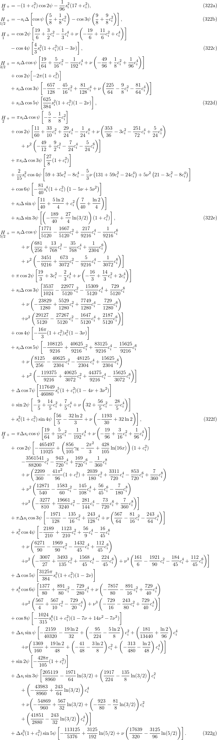
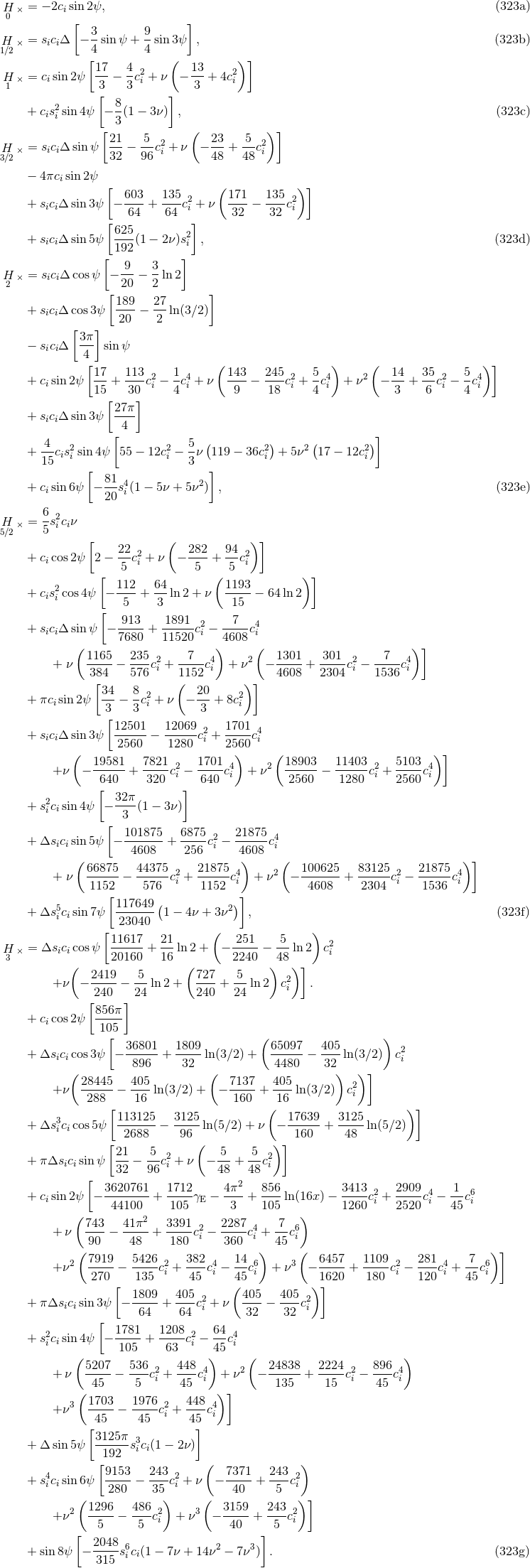
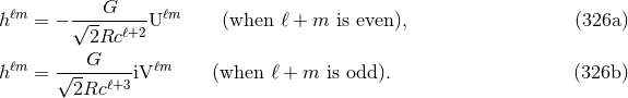
A useful fact to remember is that for non-spinning binaries, the mode  is entirely given by the
mass multipole moment
is entirely given by the
mass multipole moment  when
when  is even, and by the current one
  when
when  is odd.
This is valid in general for non-spinning binaries, regardless of the orbit being quasi-circular or elliptical.
The important point is only that the motion of the two particles must be planar, i.e., takes place in a fixed
plane. This is the case if the particles are non-spinning, but this will also be the case if, more generally, the
spins are aligned or anti-aligned with the orbital angular momentum, since there is no orbital precession
in this case. Thus, for any “planar” binaries, Eq. (73*) splits to (see Ref. [197*] for a proof)
is odd.
This is valid in general for non-spinning binaries, regardless of the orbit being quasi-circular or elliptical.
The important point is only that the motion of the two particles must be planar, i.e., takes place in a fixed
plane. This is the case if the particles are non-spinning, but this will also be the case if, more generally, the
spins are aligned or anti-aligned with the orbital angular momentum, since there is no orbital precession
in this case. Thus, for any “planar” binaries, Eq. (73*) splits to (see Ref. [197*] for a proof)
Let us factorize out in all the modes an overall coefficient including the appropriate phase factor
 , where we recall that
  denotes the tail-distorted phase introduced in Eq. (321*), and such that
the dominant mode with
denotes the tail-distorted phase introduced in Eq. (321*), and such that
the dominant mode with  conventionally starts with one at the Newtonian order. We thus
pose
conventionally starts with one at the Newtonian order. We thus
pose

 . We assume
  ; the modes having
  are easily deduced using
 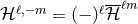 . The dominant mode
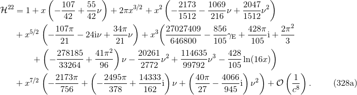
  , which is primarily
important for numerical relativity comparisons, is known at 3.5PN order and reads [74*, 197]
, which is primarily
important for numerical relativity comparisons, is known at 3.5PN order and reads [74*, 197]
 and
and  also known at 3.5PN order
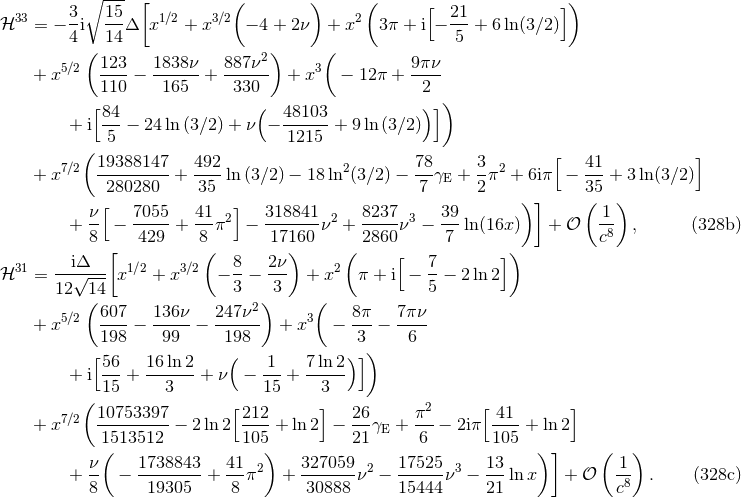
The other modes are known with a precision consistent with 3PN order in the full waveform [74]:
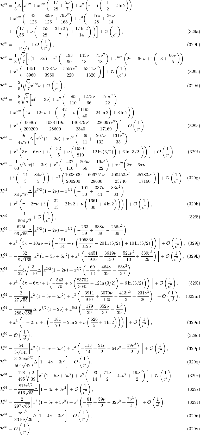
Notice that the modes with  are zero except for the DC (zero-frequency) non-linear memory
contributions. We already know that this effect arises at Newtonian order [see Eq. (322a)], hence the non
zero values of the modes
are zero except for the DC (zero-frequency) non-linear memory
contributions. We already know that this effect arises at Newtonian order [see Eq. (322a)], hence the non
zero values of the modes  and
and  . See Ref. [189] for the DC memory contributions in the higher
modes having
. See Ref. [189] for the DC memory contributions in the higher
modes having  .
.
With the 3PN approximation all the modes with  can be considered as merely Newtonian. We
give here the general Newtonian leading order expressions of any mode with arbitrary
can be considered as merely Newtonian. We
give here the general Newtonian leading order expressions of any mode with arbitrary  and non-zero
  (see the derivation in [272]):
in which we employ the function 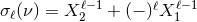 , also given by Eqs. (305).
 |
 |
 |