10 Eccentric Compact Binaries
Inspiralling compact binaries are usually modelled as moving in quasi-circular orbits since gravitational radiation reaction circularizes the orbit towards the late stages of inspiral [340*, 339*], as we discussed in Section 1.2. Nevertheless, there is an increased interest in inspiralling binaries moving in quasi-eccentric orbits. Astrophysical scenarios currently exist which lead to binaries with non-zero eccentricity in the gravitational-wave detector bandwidth, both terrestrial and space-based. For instance, inner binaries of hierarchical triplets undergoing Kozai oscillations [283, 300] could not only merge due to gravitational radiation reaction but a fraction of them should have non negligible eccentricities when they enter the sensitivity band of advanced ground based interferometers [419]. On the other hand the population of stellar mass binaries in globular clusters is expected to have a thermal distribution of eccentricities [32]. In a study of the growth of intermediate black holes [235*] in globular clusters it was found that the binaries have eccentricities between 0.1 and 0.2 in the eLISA bandwidth. Though, supermassive black hole binaries are powerful gravitational wave sources for eLISA, it is not known if they would be in quasi-circular or quasi-eccentric orbits. If a Kozai mechanism is at work, these supermassive black hole binaries could be in highly eccentric orbits and merge within the Hubble time [40]. Sources of the kind discussed above provide the prime motivation for investigating higher post-Newtonian order modelling for quasi-eccentric binaries.
10.1 Doubly periodic structure of the motion of eccentric binaries
In Section 7.3 we have given the equations of motion of non-spinning compact binary systems in the frame of the center-of-mass for general orbits at the 3PN and even 3.5PN order. We shall now investigate (in this section and the next one) the explicit solution to those equations. In particular, let us discuss the general “doubly-periodic” structure of the post-Newtonian solution, closely following Refs. [142, 143*, 149*].
The 3PN equations of motion admit, when neglecting the radiation reaction terms at 2.5PN order, ten
first integrals of the motion corresponding to the conservation of energy, angular momentum,
linear momentum, and center of mass position. When restricted to the frame of the center of
mass, the equations admit four first integrals associated with the energy  and the angular
momentum vector
and the angular
momentum vector  , given in harmonic coordinates at 3PN order by Eqs. (4.8) – (4.9) of
Ref. [79].
, given in harmonic coordinates at 3PN order by Eqs. (4.8) – (4.9) of
Ref. [79].
The motion takes place in the plane orthogonal to  . Denoting by
  the binary’s orbital
separation in that plane, and by
the binary’s orbital
separation in that plane, and by  the relative velocity, we find that
  and
and  are functions
of
are functions
of  ,
,  ,
,  and
and  . We adopt polar coordinates
  in the orbital plane, and express
  and the norm
  , thanks to
  , as some explicit functions of
  ,
,  and
and  . The latter functions can be inverted by means of a straightforward post-Newtonian
iteration to give
. The latter functions can be inverted by means of a straightforward post-Newtonian
iteration to give  and
and  in terms of
  and the constants of motion
  and
and  . Hence,
where  and
and  denote certain polynomials in
  , the degree of which depends on the
post-Newtonian approximation in question; for instance it is seventh degree for both
, the degree of which depends on the
post-Newtonian approximation in question; for instance it is seventh degree for both  and
and  at 3PN
order [312*]. The various coefficients of the powers of
at 3PN
order [312*]. The various coefficients of the powers of  are themselves polynomials in
  and
and  , and
also, of course, depend on the total mass
, and
also, of course, depend on the total mass  and symmetric mass ratio
  . In the case of bounded
elliptic-like motion, one can prove [143] that the function
. In the case of bounded
elliptic-like motion, one can prove [143] that the function  admits two real roots, say
  and
and  such that
  , which admit some non-zero finite Newtonian limits when
  , and represent
respectively the radii of the orbit’s periastron (p) and apastron (a). The other roots are complex and tend
to zero when
, and represent
respectively the radii of the orbit’s periastron (p) and apastron (a). The other roots are complex and tend
to zero when  .
.
Let us consider a given binary’s orbital configuration, fully specified by some
values of the integrals of motion  and
and  corresponding to quasi-elliptic
motion.70
The binary’s orbital period, or time of return to the periastron, is obtained by integrating the radial motion
as
corresponding to quasi-elliptic
motion.70
The binary’s orbital period, or time of return to the periastron, is obtained by integrating the radial motion
as
![∫ ra dr P = 2 ∘-----. (332 ) rp ℛ [r]](article2487x.gif)
 ) of the advance of the periastron per
orbital revolution,
which is such that the precession of the periastron per period is given by
) of the advance of the periastron per
orbital revolution,
which is such that the precession of the periastron per period is given by ![∫ ra K = -1 dr∘-𝒮[r]-, (333 ) π rp ℛ [r]](article2489x.gif)
 . As
. As  tends to one in the limit
  (as is easily checked from the usual Newtonian solution),
it is often convenient to pose
(as is easily checked from the usual Newtonian solution),
it is often convenient to pose  , which will then entirely describe the relativistic
precession.
, which will then entirely describe the relativistic
precession.
Let us then define the mean anomaly  and the mean motion
  by
by
Here  denotes the instant of passage to the periastron. For a given value of the mean anomaly
  ,
the orbital separation
,
the orbital separation  is obtained by inversion of the integral equation
![∫ r --ds--- ℓ = n ∘ -----. (335 ) rp ℛ [s]](article2500x.gif)
 which is a periodic function in
  with period
  . The orbital phase
 is then obtained in terms of the mean anomaly
  by integrating the angular motion as
where
by integrating the angular motion as
where ![∫ ℓ 1- ϕ = ϕp + n 0 dl𝒮 [r(l)], (336 )](article2506x.gif)
 denotes the value of the phase at the instant
  . We may define the origin of the orbital phase
at the ascending node
. We may define the origin of the orbital phase
at the ascending node  with respect to some observer. In the particular case of a circular orbit,
 , the phase evolves linearly with time,
 ![ϕ˙= 𝒮 [r] = Ω](article2511x.gif) , where
, where  is the orbital frequency of the
circular orbit given by
In the general case of a non-circular orbit it is convenient to keep that definition
is the orbital frequency of the
circular orbit given by
In the general case of a non-circular orbit it is convenient to keep that definition 
 and to
explicitly introduce the linearly growing part of the orbital phase (336*) by writing it in the
form
and to
explicitly introduce the linearly growing part of the orbital phase (336*) by writing it in the
form

Here  denotes a certain function of the mean anomaly which is periodic in
  with period
  ,
hence periodic in time with period
,
hence periodic in time with period  . According to Eq. (336*) this function is given in terms of the mean
anomaly
. According to Eq. (336*) this function is given in terms of the mean
anomaly  by
by
![1 ∫ ℓ W (ℓ) = -- dl(𝒮 [r(l)] − Ω ). (339 ) n 0](article2521x.gif)
 is periodic with period
  , and the periastron
advance
, and the periastron
advance  is periodic with period
  . Notice however that, though standard, the term “doubly
periodic” is misleading since the motion in physical space is not periodic in general. The radial
motion
. Notice however that, though standard, the term “doubly
periodic” is misleading since the motion in physical space is not periodic in general. The radial
motion  is periodic with period
  while the angular motion
  is periodic [modulo
 ] with period
  where
where  . Only when the two periods are commensurable,
i.e., when
. Only when the two periods are commensurable,
i.e., when  where
where  , is the motion periodic in physical space (with period
 ).
).
10.2 Quasi-Keplerian representation of the motion
The quasi-Keplerian (QK) representation of the motion of compact binaries is an elegant formulation of the
solution of the 1PN equations of motion parametrized by the eccentric anomaly  (entering a specific
generalization of Kepler’s equation) and depending on various orbital elements, such as three types of
eccentricities. It was introduced by Damour & Deruelle [149*, 150] to study the problem of binary pulsar
timing data including relativistic corrections at the 1PN order, where the relativistic periastron precession
complicates the simpler Keplerian solution.
(entering a specific
generalization of Kepler’s equation) and depending on various orbital elements, such as three types of
eccentricities. It was introduced by Damour & Deruelle [149*, 150] to study the problem of binary pulsar
timing data including relativistic corrections at the 1PN order, where the relativistic periastron precession
complicates the simpler Keplerian solution.
In the QK representation the radial motion is given in standard parametric form as
where
 is the eccentric anomaly, with
  and
and  denoting two constants representing the semi-major
axis of the orbit and its eccentricity. However, these constants are labelled after the radial coordinate
denoting two constants representing the semi-major
axis of the orbit and its eccentricity. However, these constants are labelled after the radial coordinate  to
remember that they enter (by definition) into the radial equation; in particular
to
remember that they enter (by definition) into the radial equation; in particular  will differ from other
kinds of eccentricities
will differ from other
kinds of eccentricities  and
and  . The “time” eccentricity
  enters the Kepler equation which at the
1PN order takes the usual form
where the mean anomaly is proportional to the time elapsed since the instant
enters the Kepler equation which at the
1PN order takes the usual form
where the mean anomaly is proportional to the time elapsed since the instant 
 of passage at the
periastron,
of passage at the
periastron,  where
where  is the mean motion and
  is the orbital period; see
Eqs. (334). The “angular” eccentricity
is the orbital period; see
Eqs. (334). The “angular” eccentricity  enters the equation for the angular motion at 1PN order which
is written in the form
where the true anomaly
enters the equation for the angular motion at 1PN order which
is written in the form
where the true anomaly 
 is defined by71
The constant
is defined by71
The constant ![[ ( 1 + e )1∕2 u ] v ≡ 2arctan ----ϕ-- tan -- . (343 ) 1 − eϕ 2](article2554x.gif)
 is the advance of periastron per orbital revolution defined by Eq. (333*); it may be
written as
is the advance of periastron per orbital revolution defined by Eq. (333*); it may be
written as  where
where  is the angle of return to the periastron.
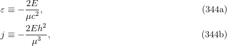
Crucial to the formalism are the explicit expressions for the orbital elements  ,
,  ,
,  ,
,  ,
,
 and
and  in terms of the conserved energy
  and angular momentum
  of the orbit.
For convenience we introduce two dimensionless parameters directly linked to
of the orbit.
For convenience we introduce two dimensionless parameters directly linked to  and
and  by
by
where  is the reduced mass with
  the total mass (recall that
  for
bound orbits) and we have used the intermediate standard notation
for
bound orbits) and we have used the intermediate standard notation  . The equations
to follow will then appear as expansions in powers of the small post-Newtonian parameter
. The equations
to follow will then appear as expansions in powers of the small post-Newtonian parameter
 ,72
with coefficients depending on
,72
with coefficients depending on  and the dimensionless reduced mass ratio
  ; notice that the parameter
 is at Newtonian order,
  . We have [149*]
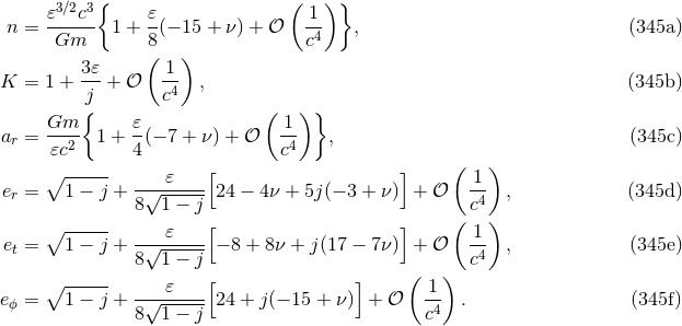
The dependence of such relations on the coordinate system in use will be discussed later. Notice the
interesting point that there is no dependence of the mean motion  and the radial semi-major axis
  on the angular momentum
  up to the 1PN order; such dependence will start only at 2PN order, see e.g.,
Eq. (347a).
up to the 1PN order; such dependence will start only at 2PN order, see e.g.,
Eq. (347a).
The above QK representation of the compact binary motion at 1PN order has been generalized at the
2PN order in Refs. [170*, 379*, 420*], and at the 3PN order by Memmesheimer, Gopakumar &
Schäfer [312*]. The construction of a generalized QK representation at 3PN order exploits the fact that the
radial equation given by Eq. (331a) is a polynomial in  (of seventh degree at 3PN order). However,
this is true only in coordinate systems avoiding the appearance of terms with the logarithm
(of seventh degree at 3PN order). However,
this is true only in coordinate systems avoiding the appearance of terms with the logarithm  ; the
presence of logarithms in the standard harmonic (SH) coordinates at the 3PN order will obstruct the
construction of the QK parametrization. Therefore Ref. [312*] obtained it in the ADM coordinate system
and also in the modified harmonic (MH) coordinates, obtained by applying the gauge transformation given
in Eq. (204*) on the SH coordinates. The equations of motion in the center-of-mass frame in MH coordinates
have been given in Eqs. (222); see also Ref. [9*] for details about the transformation between SH and MH
coordinates.
; the
presence of logarithms in the standard harmonic (SH) coordinates at the 3PN order will obstruct the
construction of the QK parametrization. Therefore Ref. [312*] obtained it in the ADM coordinate system
and also in the modified harmonic (MH) coordinates, obtained by applying the gauge transformation given
in Eq. (204*) on the SH coordinates. The equations of motion in the center-of-mass frame in MH coordinates
have been given in Eqs. (222); see also Ref. [9*] for details about the transformation between SH and MH
coordinates.
At the 3PN order the radial equation in ADM or MH coordinates is still given by Eq. (340*). However, the Kepler equation (341*) and angular equation (342*) acquire extra contributions and now become
in which the true anomaly  is still given by Eq. (343*). The new orbital elements
 ,
,  ,
,  ,
,  ,
,  ,
,  ,
,  and
and  parametrize the 2PN and 3PN relativistic
corrections.73
All the orbital elements are now to be related, similarly to Eqs. (345), to the constants
parametrize the 2PN and 3PN relativistic
corrections.73
All the orbital elements are now to be related, similarly to Eqs. (345), to the constants  and
and  with
3PN accuracy in a given coordinate system. Let us make clear that in different coordinate systems such as
MH and ADM coordinates, the QK representation takes exactly the same form as given by Eqs. (340*) and
(346). But, the relations linking the various orbital elements
with
3PN accuracy in a given coordinate system. Let us make clear that in different coordinate systems such as
MH and ADM coordinates, the QK representation takes exactly the same form as given by Eqs. (340*) and
(346). But, the relations linking the various orbital elements  ,
,  ,
,  ,
,  ,
,  ,
,  ,
,
 to
to  and
and  or
or  and
and  , are different, with the notable exceptions of
  and
and
 .
.
Indeed, an important point related to the use of gauge invariant variables in the elliptical orbit case is
that the functional forms of the mean motion  and periastron advance
  in terms of the gauge
invariant variables
in terms of the gauge
invariant variables  and
and  are identical in different coordinate systems like the MH and ADM
coordinates [170*]. Their explicit expressions at 3PN order read
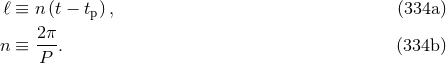
are identical in different coordinate systems like the MH and ADM
coordinates [170*]. Their explicit expressions at 3PN order read
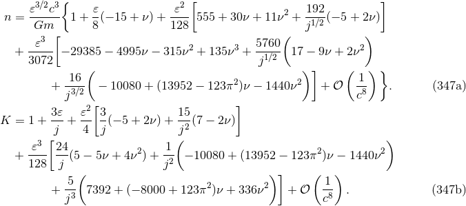
Because of their gauge invariant meaning, it is natural to use  and
and  as two independent
gauge-invariant variables in the general orbit case. Actually, instead of working with the mean motion
as two independent
gauge-invariant variables in the general orbit case. Actually, instead of working with the mean motion  it
is often preferable to use the orbital frequency
it
is often preferable to use the orbital frequency  which has been defined for general quasi-elliptic orbits in
Eq. (337*). Moreover we can pose
which has been defined for general quasi-elliptic orbits in
Eq. (337*). Moreover we can pose

 used in the circular orbit
case. The use of
used in the circular orbit
case. The use of  as an independent parameter will thus facilitate the straightforward reading out and
check of the circular orbit limit. The parameter
as an independent parameter will thus facilitate the straightforward reading out and
check of the circular orbit limit. The parameter  is related to the energy and angular momentum
variables
is related to the energy and angular momentum
variables  and
and  up to 3PN order by
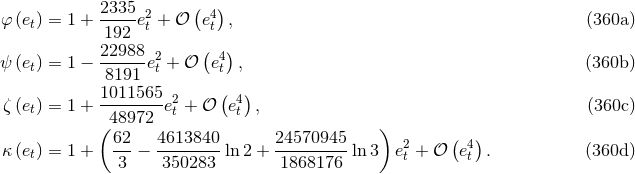
Besides the very useful gauge-invariant quantities  ,
,  and
and  , the other orbital elements
  ,
,
 ,
,  ,
,  ,
,  ,
,  ,
,  ,
,  ,
,  ,
,  ,
,  ,
,  parametrizing Eqs. (340*) and (346) are not
gauge invariant; their expressions in terms of
parametrizing Eqs. (340*) and (346) are not
gauge invariant; their expressions in terms of  and
and  depend on the coordinate system in use. We refer
to Refs. [312*, 9*] for the full expressions of all the orbital elements at 3PN order in both MH and ADM
coordinate systems. Here, for future use, we only give the expression of the time eccentricity
depend on the coordinate system in use. We refer
to Refs. [312*, 9*] for the full expressions of all the orbital elements at 3PN order in both MH and ADM
coordinate systems. Here, for future use, we only give the expression of the time eccentricity  (squared)
in MH coordinates:
(squared)
in MH coordinates:
Again, with our notation (344), this appears as a post-Newtonian expansion in the small parameter
 with fixed “Newtonian” parameter
  .
.
In the case of a circular orbit, the angular momentum variable, say  , is related to the constant of
energy
, is related to the constant of
energy  by the 3PN gauge-invariant expansion
![( ) ( 2) ( [ ] 2 3) ( ) j = 1 + 9-+ ν- 𝜀+ 81-− 2ν + ν-- 𝜀2+ 945- + − 7699-+ 41π2 ν + ν--+ ν-- 𝜀3+ 𝒪 1- . circ 4 4 16 16 64 192 32 2 64 c8](article2658x.gif)
This permits to reduce various quantities to circular orbits, for instance, the periastron advance is found to be well defined in the limiting case of a circular orbit, and is given at 3PN order in terms of the PN parameter (230*) [or (348*)] by
![( 27 ) ( 135 [ 649 123 ] ) ( 1 ) Kcirc = 1 + 3x + ---− 7 ν x2 + ----+ − ----+ ---π2 ν + 7ν2 x3 + 𝒪 -8 . 2 2 4 32 c](article2659x.gif)
See Ref. [291] for a comparison between the PN prediction for the periastron advance of circular orbits and numerical calculations based on self-force theory in the small mass ratio limit.
10.3 Averaged energy and angular momentum fluxes
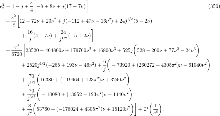
The gravitational wave energy and angular momentum fluxes from a system of two point masses in elliptic motion was first computed by Peters & Mathews [340*, 339*] at Newtonian level. The 1PN and 1.5PN corrections to the fluxes were provided in Refs. [416, 86*, 267*, 87*, 366*] and used to study the associated secular evolution of orbital elements under gravitational radiation reaction using the QK representation of the binary’s orbit at 1PN order [149]. These results were extended to 2PN order in Refs. [224*, 225] for the instantaneous terms (leaving aside the tails) using the generalized QK representation [170, 379, 420]; the energy flux and waveform were in agreement with those of Ref. [424] obtained using a different method. Arun et al. [10*, 9*, 12*] have fully generalized the results at 3PN order, including all tails and related hereditary contributions, by computing the averaged energy and angular momentum fluxes for quasi-elliptical orbits using the QK representation at 3PN order [312], and deriving the secular evolution of the orbital elements under 3PN gravitational radiation reaction.74
The secular evolution of orbital elements under gravitational radiation reaction is in principle only the starting point for constructing templates for eccentric binary orbits. To go beyond the secular evolution one needs to include in the evolution of the orbital elements, besides the averaged contributions in the fluxes, the terms rapidly oscillating at the orbital period. An analytic approach, based on an improved method of variation of constants, has been discussed in Ref. [153*] for dealing with this issue at the leading 2.5PN radiation reaction order.
The generalized QK representation of the motion discussed in Section 10.2 plays a crucial role in
the procedure of averaging the energy and angular momentum fluxes  and
and  over one
orbit.75
Actually the averaging procedure applies to the “instantaneous” parts of the fluxes, while the “hereditary”
parts are treated separately for technical reasons [10*, 9*, 12*]. Following the decomposition (308*) we pose
over one
orbit.75
Actually the averaging procedure applies to the “instantaneous” parts of the fluxes, while the “hereditary”
parts are treated separately for technical reasons [10*, 9*, 12*]. Following the decomposition (308*) we pose
 where the hereditary part of the energy flux is composed of tails and tail-of-tails. For
the angular momentum flux one needs also to include a contribution from the memory effect [12*]. We thus
have to compute for the instantaneous part
where the hereditary part of the energy flux is composed of tails and tail-of-tails. For
the angular momentum flux one needs also to include a contribution from the memory effect [12*]. We thus
have to compute for the instantaneous part

 .
.
Thanks to the QK representation, we can express  , which is initially a function of
the natural variables
, which is initially a function of
the natural variables  ,
,  and
and  , as a function of the varying eccentric anomaly
  ,
and depending on two constants: The frequency-related parameter
,
and depending on two constants: The frequency-related parameter  defined by (348*), and
the “time” eccentricity
defined by (348*), and
the “time” eccentricity  given by (350). To do so one must select a particular coordinate
system – the MH coordinates for instance. The choice of
given by (350). To do so one must select a particular coordinate
system – the MH coordinates for instance. The choice of  rather than
  (say) is a matter
of convenience; since
(say) is a matter
of convenience; since  appears in the Kepler-like equation (346a) at leading order, it will
directly be dealt with when averaging over one orbit. We note that in the expression of the
energy flux at the 3PN order there are some logarithmic terms of the type
appears in the Kepler-like equation (346a) at leading order, it will
directly be dealt with when averaging over one orbit. We note that in the expression of the
energy flux at the 3PN order there are some logarithmic terms of the type  even
in MH coordinates. Indeed, as we have seen in Section 7.3, the MH coordinates permit the
removal of the logarithms
even
in MH coordinates. Indeed, as we have seen in Section 7.3, the MH coordinates permit the
removal of the logarithms  in the equations of motion, where
  is the UV scale
associated with Hadamard’s self-field regularization [see Eq. (221*)]; however there are still
some logarithms
is the UV scale
associated with Hadamard’s self-field regularization [see Eq. (221*)]; however there are still
some logarithms  which involve the IR constant
  entering the definition of the
multipole moments for general sources, see Theorem 6 where the finite part
entering the definition of the
multipole moments for general sources, see Theorem 6 where the finite part  contains the
regularization factor (42*). As a result we find that the general structure of
contains the
regularization factor (42*). As a result we find that the general structure of  (and similarly for
 , the norm of the angular momentum flux) consists of a finite sum of terms of the type

 has been inserted to prepare for the orbital average (351*). The coefficients
  ,
,  and
and  are straightforwardly computed using the QK parametrization as functions of
  and
the time eccentricity
and
the time eccentricity  . The
. The  ’s correspond to 2.5PN radiation-reaction terms and will
play no role, while the
’s correspond to 2.5PN radiation-reaction terms and will
play no role, while the  ’s correspond to the logarithmic terms
  arising at the
3PN order. For convenience the dependence on the constant
arising at the
3PN order. For convenience the dependence on the constant  has been included into the
coefficients
has been included into the
coefficients  ’s. To compute the average we dispose of the following integration formulas
(
’s. To compute the average we dispose of the following integration formulas
( )76
)76
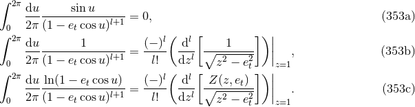
In the right-hand sides of Eqs. (353b) and (353c) we have to differentiate  times with respect to the
intermediate variable
times with respect to the
intermediate variable  before applying
  . The equation (353c), necessary for dealing with the
logarithmic terms, contains the not so trivial function
. The equation (353c), necessary for dealing with the
logarithmic terms, contains the not so trivial function
![[ ∘1--−-e2 + 1] [ ∘1--−-e2 − 1 ] Z (z,et) = ln -------t----- + 2 ln 1 + ----∘--t----- . (354 ) 2 z + z2 − e2t](article2702x.gif)
 and vanishes after averaging since it involves only odd functions
of
and vanishes after averaging since it involves only odd functions
of  .
.
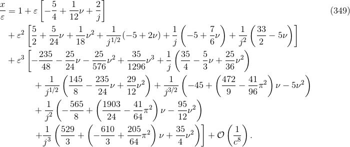
Finally, after implementing all the above integrations, the averaged instantaneous energy flux in MH coordinates at the 3PN order is obtained in the form [9]
where we recall that the post-Newtonian parameter
 is defined by (348*). The various instantaneous
post-Newtonian pieces depend on the symmetric mass ratio
is defined by (348*). The various instantaneous
post-Newtonian pieces depend on the symmetric mass ratio  and the time eccentricity
  in MH
coordinates as
in MH
coordinates as
The Newtonian coefficient  is nothing but the Peters & Mathews [340] enhancement function of
eccentricity that enters in the orbital gravitational radiation decay of the binary pulsar; see Eq. (11*). For
ease of presentation we did not add a label on
is nothing but the Peters & Mathews [340] enhancement function of
eccentricity that enters in the orbital gravitational radiation decay of the binary pulsar; see Eq. (11*). For
ease of presentation we did not add a label on  to indicate that it is the time eccentricity in MH
coordinates; such MH-coordinates
to indicate that it is the time eccentricity in MH
coordinates; such MH-coordinates  is given by Eq. (350). Recall that on the contrary
  is gauge
invariant, so no such label is required on it.
is gauge
invariant, so no such label is required on it.
The last term in the 3PN coefficient is proportional to some logarithm which directly arises from the integration formula (353c). Inside the logarithm we have posed
exhibiting an explicit dependence upon the arbitrary length scale
 ; we recall that
  was introduced
in the formalism through Eq. (42*). Only after adding the hereditary contribution to the 3PN energy flux
can we check the required cancellation of the constant
was introduced
in the formalism through Eq. (42*). Only after adding the hereditary contribution to the 3PN energy flux
can we check the required cancellation of the constant  . The hereditary part is made of tails and
tails-of-tails, and is of the form
where the post-Newtonian pieces, only at the 1.5PN, 2.5PN and 3PN orders, read [10*]
. The hereditary part is made of tails and
tails-of-tails, and is of the form
where the post-Newtonian pieces, only at the 1.5PN, 2.5PN and 3PN orders, read [10*]

where  ,
,  ,
,  ,
,  and
and  are certain “enhancement” functions of the
eccentricity.
are certain “enhancement” functions of the
eccentricity.
Among them the four functions  ,
,  ,
,  and
and  appearing in Eqs. (359) do not
admit analytic closed-form expressions. They have been obtained in Refs. [10*] (extending Ref. [87*]) in the
form of infinite series made out of quadratic products of Bessel functions. Numerical plots of these four
enhancement factors as functions of eccentricity
appearing in Eqs. (359) do not
admit analytic closed-form expressions. They have been obtained in Refs. [10*] (extending Ref. [87*]) in the
form of infinite series made out of quadratic products of Bessel functions. Numerical plots of these four
enhancement factors as functions of eccentricity  have been provided in Ref. [10*]; we give
in Figure 3* the graph of the function
have been provided in Ref. [10*]; we give
in Figure 3* the graph of the function  which enters the dominant 1.5PN tail term in
Eq. (358*).
which enters the dominant 1.5PN tail term in
Eq. (358*).
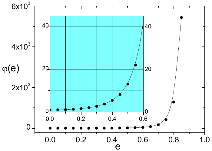
 with the eccentricity
  . This function agrees
with the numerical calculation of Ref. [87*] modulo a trivial rescaling with the Peters–Mathews
function (356a). The inset graph is a zoom of the function at a smaller scale. The dots represent the
numerical computation and the solid line is a fit to the numerical points. In the circular orbit limit
we have
. This function agrees
with the numerical calculation of Ref. [87*] modulo a trivial rescaling with the Peters–Mathews
function (356a). The inset graph is a zoom of the function at a smaller scale. The dots represent the
numerical computation and the solid line is a fit to the numerical points. In the circular orbit limit
we have  .
. Furthermore their leading correction term  in the limit of small eccentricity
  can be
obtained analytically as [10]
can be
obtained analytically as [10]
On the other hand the function  in factor of the logarithm in the 3PN piece does admit some
closed analytic form:
in factor of the logarithm in the 3PN piece does admit some
closed analytic form:
![[ ] F(et) = -----1----- 1 + 85e2t + 5171-e4t + 1751-e6t + 297-e8t . (361 ) (1 − e2t)13∕2 6 192 192 1024](article2739x.gif)
The latter analytical result is very important for checking that the arbitrary constant  disappears
from the final result. Indeed we immediately verify from comparing the last term in Eq. (356d) with
Eq. (359c) that
disappears
from the final result. Indeed we immediately verify from comparing the last term in Eq. (356d) with
Eq. (359c) that  cancels out from the sum of the instantaneous and hereditary contributions in the
3PN energy flux. This fact was already observed for the circular orbit case in Ref. [81]; see also the
discussions around Eqs. (93*) – (94*) and at the end of Section 4.2.
cancels out from the sum of the instantaneous and hereditary contributions in the
3PN energy flux. This fact was already observed for the circular orbit case in Ref. [81]; see also the
discussions around Eqs. (93*) – (94*) and at the end of Section 4.2.
Finally we can check that the correct circular orbit limit, which is given by Eq. (314), is recovered from
the sum  . The next correction of order
  when
when  can be deduced from
Eqs. (360) – (361*) in analytic form; having the flux in analytic form may be useful for studying the
gravitational waves from binary black hole systems with moderately high eccentricities, such as those
formed in globular clusters [235].
can be deduced from
Eqs. (360) – (361*) in analytic form; having the flux in analytic form may be useful for studying the
gravitational waves from binary black hole systems with moderately high eccentricities, such as those
formed in globular clusters [235].
Previously the averaged energy flux was represented using  – the gauge invariant variable (348*) –
and the time eccentricity
– the gauge invariant variable (348*) –
and the time eccentricity  which however is gauge dependent. Of course it is possible to provide a fully
gauge invariant formulation of the energy flux. The most natural choice is to express the result in terms
of the conserved energy
which however is gauge dependent. Of course it is possible to provide a fully
gauge invariant formulation of the energy flux. The most natural choice is to express the result in terms
of the conserved energy  and angular momentum
  , or, rather, in terms of the pair of
rescaled variables (
, or, rather, in terms of the pair of
rescaled variables ( ,
,  ) defined by Eqs. (344). To this end it suffices to replace
  by its
MH-coordinate expression (350) and to use Eq. (349) to re-express
by its
MH-coordinate expression (350) and to use Eq. (349) to re-express  in terms of
  and
and  .
However, there are other possible choices for a couple of gauge invariant quantities. As we have
seen the mean motion
.
However, there are other possible choices for a couple of gauge invariant quantities. As we have
seen the mean motion  and the periastron precession
  are separately gauge invariant
so we may define the pair of variables (
are separately gauge invariant
so we may define the pair of variables ( ,
,  ), where
  is given by (348*) and we pose

 reduces to the angular-momentum related variable
 in the limit
  . Note however that with the latter choices (
 ,
,  ) or (
 ,
,  ) of
gauge-invariant variables, the circular-orbit limit is not directly readable from the result; this is
why we have preferred to present it in terms of the gauge dependent couple of variables (
) of
gauge-invariant variables, the circular-orbit limit is not directly readable from the result; this is
why we have preferred to present it in terms of the gauge dependent couple of variables ( ,
,
 ).
).
As we are interested in the phasing of binaries moving in quasi-eccentric orbits in the adiabatic
approximation, we require the orbital averages not only of the energy flux  but also of the angular
momentum flux
but also of the angular
momentum flux  . Since the quasi-Keplerian orbit is planar, we only need to average the magnitude
  of the angular momentum flux. The complete computation thus becomes a generalisation of the previous
computation of the averaged energy flux requiring similar steps (see Ref. [12*]): The angular momentum flux
is split into instantaneous
of the angular momentum flux. The complete computation thus becomes a generalisation of the previous
computation of the averaged energy flux requiring similar steps (see Ref. [12*]): The angular momentum flux
is split into instantaneous  and hereditary
  contributions; the instantaneous part is averaged
using the QK representation in either MH or ADM coordinates; the hereditary part is evaluated separately
and defined by means of several types of enhancement functions of the time eccentricity
contributions; the instantaneous part is averaged
using the QK representation in either MH or ADM coordinates; the hereditary part is evaluated separately
and defined by means of several types of enhancement functions of the time eccentricity  ;
finally these are obtained numerically as well as analytically to next-to-leading order
;
finally these are obtained numerically as well as analytically to next-to-leading order  . At
this stage we dispose of both the averaged energy and angular momentum fluxes
. At
this stage we dispose of both the averaged energy and angular momentum fluxes  and
and
 .
.
The procedure to compute the secular evolution of the orbital elements under gravitational
radiation-reaction is straightforward. Differentiating the orbital elements with respect to time, and using the
heuristic balance equations, we equate the decreases of energy and angular momentum to the corresponding
averaged fluxes  and
and  at 3PN order [12]. This extends earlier analyses at previous orders:
Newtonian [339] as we have reviewed in Section 1.2; 1PN [86, 267]; 1.5PN [87, 366] and 2PN [224, 153*].
Let us take the example of the mean motion
at 3PN order [12]. This extends earlier analyses at previous orders:
Newtonian [339] as we have reviewed in Section 1.2; 1PN [86, 267]; 1.5PN [87, 366] and 2PN [224, 153*].
Let us take the example of the mean motion  . From Eq. (347a) together with the definitions (344) we
know the function
. From Eq. (347a) together with the definitions (344) we
know the function  at 3PN order, where
  and
and  are the orbit’s constant energy and angular
momentum. Thus,
are the orbit’s constant energy and angular
momentum. Thus,

have already been used at Newtonian order in Eqs. (9). Although heuristically assumed at 3PN order, they have been proved through 1.5PN order in Section 5.4. With the averaged fluxes known through 3PN order, we obtain the 3PN averaged evolution equation as
We recall that this gives only the slow secular evolution under gravitational radiation reaction for eccentric orbits. The complete evolution includes also, superimposed on the averaged adiabatic evolution, some fast but smaller post-adiabatic oscillations at the orbital time scale [153, 279].
 |
 |
 |