List of Figures
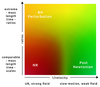 |
Figure 1:
Range of various approximation tools (“UR” stands for ultra-relativistic). NR is mostly limited by resolution issues and therefore by possible different scales in the problem. |
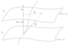 |
Figure 2:
Illustration of two hypersurfaces of a foliation  . Lapse . Lapse  and shift and shift  are defined
by the relation of the timelike unit normal field are defined
by the relation of the timelike unit normal field  and the basis vector and the basis vector  associated with the
coordinate associated with the
coordinate  . Note that . Note that  and, hence, the shift vector and, hence, the shift vector  is tangent to is tangent to  . . |
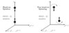 |
Figure 3:
 -dimensional representation of head-on collisons for spinless BHs, with isometry group -dimensional representation of head-on collisons for spinless BHs, with isometry group
 (left), and non-head-on collisons for BHs spinning in the orbital plane, with isometry
group (left), and non-head-on collisons for BHs spinning in the orbital plane, with isometry
group  (right). Image reproduced with permission from [841], copyright by APS. (right). Image reproduced with permission from [841], copyright by APS. |
 |
Figure 4:
Illustration of mesh refinement for a BH binary with one spatial dimension suppressed. Around each BH (marked by the spherical AH), two nested boxes are visible. These are immersed within one large, common grid or refinement level. |
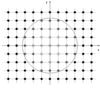 |
Figure 5:
Illustration of singularity excision. The small circles represent vertices of a numerical grid on a two-dimensional cross section of the computational domain containing the spacetime singularity, in this case at the origin. A finite region around the singularity but within the event horizon (large circle) is excluded from the numerical evolution (white circles). Gray circles represent the excision boundary where function values can be obtained through regular evolution in time using sideways derivative operators as appropriate (e.g., [630]) or regular update with spectral methods (e.g., [677, 678]), or through extrapolation (e.g., [703, 723]). The regular evolution of exterior grid points (black circles) is performed with standard techniques using information also on the excision boundary. |
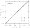 |
Figure 6:
Illustration of the conjectured mass-scaling relation (172*). The data refer to three separate one-parameter variations of the pulse shape (171*). The constants  and and  are chosen to
normalize the ranges of the abscissa and place the data point corresponding to the smallest BH in
each family at the origin. Image reproduced with permission from [212], copyright by APS. are chosen to
normalize the ranges of the abscissa and place the data point corresponding to the smallest BH in
each family at the origin. Image reproduced with permission from [212], copyright by APS. |
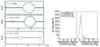 |
Figure 7:
Left panel: Embedding diagram of the AH of the perturbed black string at different stages of the evolution. The light (dark) lines denote the first (last) time from the evolution segment shown in the corresponding panel. Right panel: Dimensionless Kretschmann scalar  at the centre of
mass of a binary BH system as a function of the (areal) coordinate separation between the two BHs
in a at the centre of
mass of a binary BH system as a function of the (areal) coordinate separation between the two BHs
in a  scattering, in units of scattering, in units of  . Images reproduced with permission from (left) [511]
and from (right) [587], copyright by APS. . Images reproduced with permission from (left) [511]
and from (right) [587], copyright by APS. |
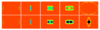 |
Figure 8:
Snapshots of the rest-mass density in the collision of fluid balls with boost factor  (upper panels) and
  (lower panels) at the initial time, shortly after collision, at the time
corresponding to the formation of separate horizons in the (lower panels) at the initial time, shortly after collision, at the time
corresponding to the formation of separate horizons in the  case, and formation of a common
horizon (for case, and formation of a common
horizon (for  ) and at late time in the dispersion ( ) and at late time in the dispersion ( ) or ringdown ( ) or ringdown ( ) phase.
Image reproduced with permission from [288], copyright by APS. ) phase.
Image reproduced with permission from [288], copyright by APS. |
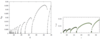 |
Figure 9:
Instability against BH formation in AdS (left panel) and Minkowski enclosed in a cavity (right panel). In both panels, the horizontal axis represents the amplitude of the initial (spherically symmetric) scalar field perturbation. The vertical axis represents the size of the BH formed. Perturbations with the largest plotted amplitude collapse to form a BH. As the amplitude of the perturbation is decreased so does the size of the BH, which tends to zero at a first threshold amplitude. Below this energy, no BH is formed in the first generation collapse and the scalar perturbation scatters towards the boundary. But since the spacetime behaves like a cavity, the scalar perturbation is reflected off the boundary and re-collapses, forming now a BH during the second generation collapse. At smaller amplitudes a second, third, etc, threshold amplitudes are found. The left (right) panel shows ten (five) generations of collapse. Near the threshold amplitudes, critical behavior is observed. Images reproduced with permission from (left) [108] and from (right) [537], copyright by APS. |
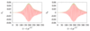 |
Figure 10:
(a) and (b):  and and  modes of gravitational waveform (solid curve) from an unstable
six-dimensional BH with modes of gravitational waveform (solid curve) from an unstable
six-dimensional BH with  as a function of a retarded time defined by as a function of a retarded time defined by  , where , where  is the coordinate distance from the center. Image reproduced with permission from [700], copyright
by APS.
is the coordinate distance from the center. Image reproduced with permission from [700], copyright
by APS. |
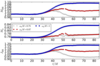 |
Figure 11:
Evolution of a highly spinning BH (  ) during interaction with different
frequency GW packets, each with initial mass ) during interaction with different
frequency GW packets, each with initial mass  . Shown (in units where . Shown (in units where  ) are the
mass, irreducible mass, and angular momentum of the BH as inferred from AH properties. Image
reproduced with permission from [289], copyright by APS. ) are the
mass, irreducible mass, and angular momentum of the BH as inferred from AH properties. Image
reproduced with permission from [289], copyright by APS. |
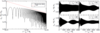 |
Figure 12:
Massive scalar field (nonlinear) evolution of the spacetime of an initially non-rotating BH, with  . Left panel: Evolution of a spherically symmetric . Left panel: Evolution of a spherically symmetric  scalar waveform,
measured at scalar waveform,
measured at  , with , with  the initial BH mass. In addition to the numerical data (black
solid curve) we show a fit to the late-time tail (red dashed curve) with the initial BH mass. In addition to the numerical data (black
solid curve) we show a fit to the late-time tail (red dashed curve) with  , in excellent agreement
with linearized analysis. Right panel: The dipole signal resulting from the evolution of an , in excellent agreement
with linearized analysis. Right panel: The dipole signal resulting from the evolution of an  massive scalar field around a non-rotating BH. The waveforms, extracted at different radii
  exhibit pronounced beating patterns caused by interference of different overtones. The critical feature
is however, that these are extremely long-lived configurations. Image reproduced with permission
from [588], copyright by APS.
exhibit pronounced beating patterns caused by interference of different overtones. The critical feature
is however, that these are extremely long-lived configurations. Image reproduced with permission
from [588], copyright by APS. |
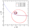 |
Figure 13:
BH trajectories in grazing collisions for  and three values of the impact
parameter corresponding to the regime of prompt merger (solid, black curve), of delayed merger
(dashed, red curve), and scattering (dotted, blue curve). Note that for each case, the trajectory of
one BH is shown only; the other BH’s location is given by symmetry across the origin. and three values of the impact
parameter corresponding to the regime of prompt merger (solid, black curve), of delayed merger
(dashed, red curve), and scattering (dotted, blue curve). Note that for each case, the trajectory of
one BH is shown only; the other BH’s location is given by symmetry across the origin. |
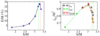 |
Figure 14:
Total energy radiated in GWs (left panel) and final dimensionless spin of the merged BH (right panel) as a function of impact parameter  for the same grazing collisions with for the same grazing collisions with  .
The vertical dashed (green) and dash-dotted (red) lines mark .
The vertical dashed (green) and dash-dotted (red) lines mark  and and  , respectively. Image
reproduced with permission from [720], copyright by APS. , respectively. Image
reproduced with permission from [720], copyright by APS. |
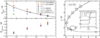 |
Figure 15:
Left panels: Scattering threshold (upper panel) and maximum radiated energy (lower panel) as a function of  . Colored “triangle” symbols pointing up and down refer to the
aligned and antialigned cases, respectively. Black “circle” symbols represent the thresholds for the
nonspinning configurations. Right panel: Trajectory of one BH for a delayed merger configuration
with anti-aligned spins . Colored “triangle” symbols pointing up and down refer to the
aligned and antialigned cases, respectively. Black “circle” symbols represent the thresholds for the
nonspinning configurations. Right panel: Trajectory of one BH for a delayed merger configuration
with anti-aligned spins  . The circles represent the BH location at equidistant intervals . The circles represent the BH location at equidistant intervals
 corresponding to the vertical lines in the inset that shows the equatorial circumference
of the BH’s AH as a function of time. corresponding to the vertical lines in the inset that shows the equatorial circumference
of the BH’s AH as a function of time. |
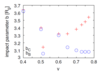 |
Figure 16:
The (red) plus and (blue) circle symbols mark scattering and merging BH configurations, respectively, in the  plane of impact parameter and collision speed, for plane of impact parameter and collision speed, for  spacetime
dimensions. spacetime
dimensions. |
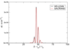 |
Figure 17:
Energy fluxes for head-on collisions of two BHs in  spacetime dimensions,
obtained with two different codes, HD-Lean [841, 797] (solid black line) and SacraND [820, 587]
(red dashed line). The BHs start off at an initial coordinate separation spacetime dimensions,
obtained with two different codes, HD-Lean [841, 797] (solid black line) and SacraND [820, 587]
(red dashed line). The BHs start off at an initial coordinate separation  . Image adapted
from [796]. . Image adapted
from [796]. |
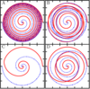 |
Figure 18:
Trajectories of BHs immersed in a scalar field bubble of different amplitudes. The BH binary consists of initially non-spinning, equal-mass BHs in quasi-circular orbit, initially separated by  , where , where  is the mass of the binary system. The scalar field bubble
surrounding the binary has a radius is the mass of the binary system. The scalar field bubble
surrounding the binary has a radius  and thickness and thickness  . Panels . Panels  correspond to
  and a zero potential amplitude and a zero potential amplitude  . Panel . Panel  corresponds
to corresponds
to  . Image reproduced with permission from [410], copyright by IOP. All
rights reserved. . Image reproduced with permission from [410], copyright by IOP. All
rights reserved. |
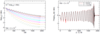 |
Figure 19:
Numerical results for a BH binary inspiralling in a scalar-field gradient  .
Left panel: dependence of the various components of the scalar radiation .
Left panel: dependence of the various components of the scalar radiation  on
the extraction radius (top to bottom: on
the extraction radius (top to bottom:  to to  in equidistant steps). The dashed line
corresponds instead to in equidistant steps). The dashed line
corresponds instead to  at the largest extraction radius. This is the dominant
mode and corresponds to the fixed-gradient boundary condition, along the at the largest extraction radius. This is the dominant
mode and corresponds to the fixed-gradient boundary condition, along the  -direction, at large
distances. Right panel: time-derivative of the scalar field at the largest and smallest extraction radii,
rescaled by radius and shifted in time. Notice how the waveforms show a clean and typical merger
pattern, and that they overlap showing that the field scales to good approximation as -direction, at large
distances. Right panel: time-derivative of the scalar field at the largest and smallest extraction radii,
rescaled by radius and shifted in time. Notice how the waveforms show a clean and typical merger
pattern, and that they overlap showing that the field scales to good approximation as  . Image
reproduced with permission from [92], copyright by APS. . Image
reproduced with permission from [92], copyright by APS. |
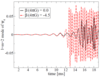 |
Figure 20:
The dominant quadrupolar component of the gravitational  scalar for an equal-mass,
non-spinning NS binary with individual baryon masses of scalar for an equal-mass,
non-spinning NS binary with individual baryon masses of  . The solid (black) curve refers
to GR, and the dashed (red) curve to a scalar-tensor theory with . The solid (black) curve refers
to GR, and the dashed (red) curve to a scalar-tensor theory with  . Image
reproduced with permission from [73], copyright by APS. . Image
reproduced with permission from [73], copyright by APS. |
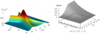 |
Figure 21:
Left panel: Collision of two shock waves in AdS5. The energy density  is represented
as a function of an (advanced) time coordinate is represented
as a function of an (advanced) time coordinate  and a longitudinal coordinate and a longitudinal coordinate  . .  defines
the amplitude of the waves. Right panel: Evolution of the scalar field in an unstable RN-AdS BH. defines
the amplitude of the waves. Right panel: Evolution of the scalar field in an unstable RN-AdS BH.
 is a radial coordinate and the AdS boundary is at is a radial coordinate and the AdS boundary is at  . Due to the instability of the BH, the
scalar density grows exponentially for . Due to the instability of the BH, the
scalar density grows exponentially for  . Then, the scalar density approaches some static
function. Images reproduced with permission from (left) [207], copyright by APS and (right) [562],
copyright by SISSA. . Then, the scalar density approaches some static
function. Images reproduced with permission from (left) [207], copyright by APS and (right) [562],
copyright by SISSA. |
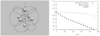 |
Figure 22:
Left: Elementary cells for the 8-BH configuration, projected to  . The marginal
surface corresponding to the BH at infinity encompasses the whole configuration. Note that the 8
cubical lattice cells are isometric after the conformal rescaling. Right: Several measures of scaling in
the eight-BH universe, as functions of proper time . The marginal
surface corresponding to the BH at infinity encompasses the whole configuration. Note that the 8
cubical lattice cells are isometric after the conformal rescaling. Right: Several measures of scaling in
the eight-BH universe, as functions of proper time  , plotted against a possible identification of the
corresponding FLRW model (see Ref. [86] for details). All the quantities have been renormalized to
their respective values at , plotted against a possible identification of the
corresponding FLRW model (see Ref. [86] for details). All the quantities have been renormalized to
their respective values at  . Images reproduced with permission from [86], copyright by IOP.
All rights reserved. . Images reproduced with permission from [86], copyright by IOP.
All rights reserved. |