2 Tests of the Foundations of Gravitation Theory

2.1 The Einstein equivalence principle

The principle of equivalence has historically played an important role in the development of gravitation theory. Newton regarded this principle as such a cornerstone of mechanics that he devoted the opening paragraph of the Principia to it. In 1907, Einstein used the principle as a basic element in his development of general relativity (GR). We now regard the principle of equivalence as the foundation, not of Newtonian gravity or of GR, but of the broader idea that spacetime is curved. Much of this viewpoint can be traced back to Robert Dicke, who contributed crucial ideas about the foundations of gravitation theory between 1960 and 1965. These ideas were summarized in his influential Les Houches lectures of 1964 [130], and resulted in what has come to be called the Einstein equivalence principle (EEP).

One elementary equivalence principle is the kind Newton had in mind when he stated that the property of a body called “mass” is proportional to the “weight”, and is known as the weak equivalence principle (WEP). An alternative statement of WEP is that the trajectory of a freely falling “test” body (one not acted upon by such forces as electromagnetism and too small to be affected by tidal gravitational forces) is independent of its internal structure and composition. In the simplest case of dropping two different bodies in a gravitational field, WEP states that the bodies fall with the same acceleration (this is often termed the Universality of Free Fall, or UFF).

The Einstein equivalence principle (EEP) is a more powerful and far-reaching concept; it states that:

1. WEP is valid.
2. The outcome of any local non-gravitational experiment is independent of the velocity of the freely-falling reference frame in which it is performed.
3. The outcome of any local non-gravitational experiment is independent of where and when in the universe it is performed.

The second piece of EEP is called local Lorentz invariance (LLI), and the third piece is called local position invariance (LPI).

For example, a measurement of the electric force between two charged bodies is a local non-gravitational experiment; a measurement of the gravitational force between two bodies (Cavendish experiment) is not.

The Einstein equivalence principle is the heart and soul of gravitational theory, for it is possible to argue convincingly that if EEP is valid, then gravitation must be a “curved spacetime” phenomenon, in other words, the effects of gravity must be equivalent to the effects of living in a curved spacetime. As a consequence of this argument, the only theories of gravity that can fully embody EEP are those that satisfy the postulates of “metric theories of gravity”, which are:

1. Spacetime is endowed with a symmetric metric.
2. The trajectories of freely falling test bodies are geodesics of that metric.
3. In local freely falling reference frames, the non-gravitational laws of physics are those written in the language of special relativity.

The argument that leads to this conclusion simply notes that, if EEP is valid, then in local freely falling frames, the laws governing experiments must be independent of the velocity of the frame (local Lorentz invariance), with constant values for the various atomic constants (in order to be independent of location). The only laws we know of that fulfill this are those that are compatible with special relativity, such as Maxwell’s equations of electromagnetism, and the standard model of particle physics. Furthermore, in local freely falling frames, test bodies appear to be unaccelerated, in other words they move on straight lines; but such “locally straight” lines simply correspond to “geodesics” in a curved spacetime (TEGP 2.3 [420*]).

General relativity is a metric theory of gravity, but then so are many others, including the Brans–Dicke theory and its generalizations. Theories in which varying non-gravitational constants are associated with dynamical fields that couple to matter directly are not metric theories. Neither, in this narrow sense, is superstring theory (see Section 2.3), which, while based fundamentally on a spacetime metric, introduces additional fields (dilatons, moduli) that can couple to material stress-energy in a way that can lead to violations, say, of WEP. It is important to point out, however, that there is some ambiguity in whether one treats such fields as EEP-violating gravitational fields, or simply as additional matter fields, like those that carry electromagnetism or the weak interactions. Still, the notion of curved spacetime is a very general and fundamental one, and therefore it is important to test the various aspects of the Einstein equivalence principle thoroughly. We first survey the experimental tests, and describe some of the theoretical formalisms that have been developed to interpret them. For other reviews of EEP and its experimental and theoretical significance, see [183, 239]; for a pedagogical review of the variety of equivalence principles, see [128].

2.1.1 Tests of the weak equivalence principle

A direct test of WEP is the comparison of the acceleration of two laboratory-sized bodies of different composition in an external gravitational field. If the principle were violated, then the accelerations of different bodies would differ. The simplest way to quantify such possible violations of WEP in a form suitable for comparison with experiment is to suppose that for a body with inertial mass , the passive gravitational mass is no longer equal to , so that in a gravitational field , the acceleration is given by . Now the inertial mass of a typical laboratory body is made up of several types of mass-energy: rest energy, electromagnetic energy, weak-interaction energy, and so on. If one of these forms of energy contributes to differently than it does to , a violation of WEP would result. One could then write

where is the internal energy of the body generated by interaction , is a dimensionless parameter that measures the strength of the violation of WEP induced by that interaction, and is the speed of light. A measurement or limit on the fractional difference in acceleration between two bodies then yields a quantity called the “Eötvös ratio” given by where we drop the subscript “I” from the inertial masses. Thus, experimental limits on place limits on the WEP-violation parameters .

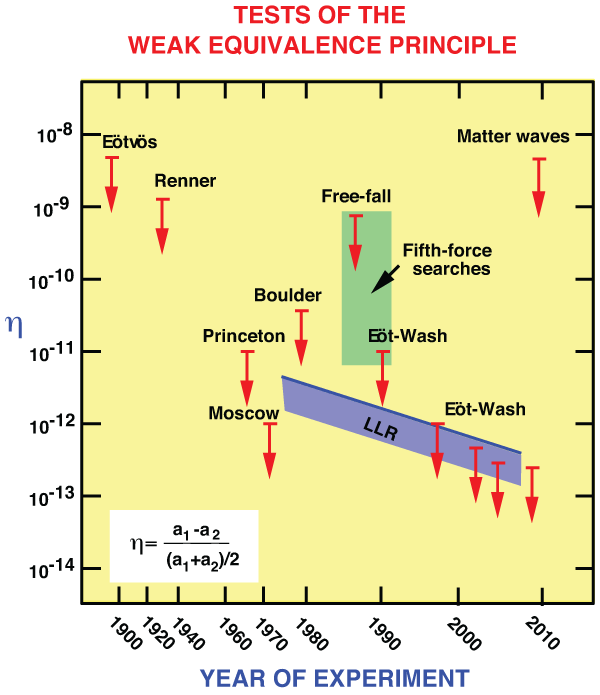
Figure 1: Selected tests of the weak equivalence principle, showing bounds on , which measures fractional difference in acceleration of different materials or bodies. The free-fall and Eöt-Wash experiments were originally performed to search for a fifth force (green region, representing many experiments). The blue band shows evolving bounds on for gravitating bodies from lunar laser ranging (LLR).

Many high-precision Eötvös-type experiments have been performed, from the pendulum experiments of Newton, Bessel, and Potter to the classic torsion-balance measurements of Eötvös [148], Dicke [131], Braginsky [65], and their collaborators (for a bibliography of experiments up to 1991, see [155*]). . In the modern torsion-balance experiments, two objects of different composition are connected by a rod or placed on a tray and suspended in a horizontal orientation by a fine wire. If the gravitational acceleration of the bodies differs, and this difference has a component perpendicular to the suspension wire, there will be a torque induced on the wire, related to the angle between the wire and the direction of the gravitational acceleration . If the entire apparatus is rotated about some direction with angular velocity , the torque will be modulated with period . In the experiments of Eötvös and his collaborators, the wire and were not quite parallel because of the centripetal acceleration on the apparatus due to the Earth’s rotation; the apparatus was rotated about the direction of the wire. In the Dicke and Braginsky experiments, was that of the Sun, and the rotation of the Earth provided the modulation of the torque at a period of 24 hr (TEGP 2.4 (a) [420*]). Beginning in the late 1980s, numerous experiments were carried out primarily to search for a “fifth force” (see Section 2.3.1), but their null results also constituted tests of WEP. In the “free-fall Galileo experiment” performed at the University of Colorado, the relative free-fall acceleration of two bodies made of uranium and copper was measured using a laser interferometric technique. The “Eöt-Wash” experiments carried out at the University of Washington used a sophisticated torsion balance tray to compare the accelerations of various materials toward local topography on Earth, movable laboratory masses, the Sun and the galaxy [379, 29*], and have reached levels of  [1*, 354, 402]. The resulting upper limits on are summarized in Figure 1*.

The recent development of atom interferometry has yielded tests of WEP, albeit to modest accuracy, comparable to that of the original Eötvös experiment. In these experiments, one measures the local acceleration of the two separated wavefunctions of an atom such as Cesium by studying the interference pattern when the wavefunctions are combined, and compares that with the acceleration of a nearby macroscopic object of different composition [278, 294]. A claim that these experiments test the gravitational redshift [294] was subsequently shown to be incorrect [439].

A number of projects are in the development or planning stage to push the bounds on even lower. The project MICROSCOPE is designed to test WEP to . It is being developed by the French space agency CNES for launch in late 2015, for a one-year mission [280]. The drag-compensated satellite will be in a Sun-synchronous polar orbit at 700 km altitude, with a payload consisting of two differential accelerometers, one with elements made of the same material (platinum), and another with elements made of different materials (platinum and titanium). Other concepts for future improvements include advanced space experiments (Galileo-Galilei, STEP, STE-QUEST), experiments on sub-orbital rockets, lunar laser ranging (see Section 4.3.1), binary pulsar observations, and experiments with anti-hydrogen. For an update on past and future tests of WEP, see the series of articles introduced by [372]. The recent discovery of a pulsar in orbit with two white-dwarf companions [332] may provide interesting new tests of WEP, because of the strong difference in composition between the neutron star and the white dwarfs, as well as precise tests of the Nordtvedt effect (see Section 4.3.1).

2.1.2 Tests of local Lorentz invariance

Although special relativity itself never benefited from the kind of “crucial” experiments, such as the perihelion advance of Mercury and the deflection of light, that contributed so much to the initial acceptance of GR and to the fame of Einstein, the steady accumulation of experimental support, together with the successful merger of special relativity with quantum mechanics, led to its acceptance by mainstream physicists by the late 1920s, ultimately to become part of the standard toolkit of every working physicist. This accumulation included

• the classic Michelson–Morley experiment and its descendents [279, 357, 208, 69*],
• the Ives–Stillwell, Rossi–Hall, and other tests of time-dilation [200, 343, 151],
• tests of whether the speed of light is independent of the velocity of the source, using both binary X-ray stellar sources and high-energy pions [67, 8],
• tests of the isotropy of the speed of light [75, 340, 234].

In addition to these direct experiments, there was the Dirac equation of quantum mechanics and its prediction of anti-particles and spin; later would come the stunningly successful relativistic theory of quantum electrodynamics. For a pedagogical review on the occasion of the 2005 centenary of special relativity, see [426].

In 2015, on the 110th anniversary of the introduction of special relativity, one might ask “what is there to test?” Special relativity has been so thoroughly integrated into the fabric of modern physics that its validity is rarely challenged, except by cranks and crackpots. It is ironic then, that during the past several years, a vigorous theoretical and experimental effort has been launched, on an international scale, to find violations of special relativity. The motivation for this effort is not a desire to repudiate Einstein, but to look for evidence of new physics “beyond” Einstein, such as apparent, or “effective” violations of Lorentz invariance that might result from certain models of quantum gravity. Quantum gravity asserts that there is a fundamental length scale given by the Planck length, , but since length is not an invariant quantity (Lorentz–FitzGerald contraction), then there could be a violation of Lorentz invariance at some level in quantum gravity. In brane-world scenarios, while physics may be locally Lorentz invariant in the higher dimensional world, the confinement of the interactions of normal physics to our four-dimensional “brane” could induce apparent Lorentz violating effects. And in models such as string theory, the presence of additional scalar, vector, and tensor long-range fields that couple to matter of the standard model could induce effective violations of Lorentz symmetry. These and other ideas have motivated a serious reconsideration of how to test Lorentz invariance with better precision and in new ways.

A simple and useful way of interpreting some of these modern experiments, called the -formalism, is to suppose that the electromagnetic interactions suffer a slight violation of Lorentz invariance, through a change in the speed of electromagnetic radiation relative to the limiting speed of material test particles (, made to take the value unity via a choice of units), in other words, (see Section 2.2.3). Such a violation necessarily selects a preferred universal rest frame, presumably that of the cosmic background radiation, through which we are moving at about  [253]. Such a Lorentz-non-invariant electromagnetic interaction would cause shifts in the energy levels of atoms and nuclei that depend on the orientation of the quantization axis of the state relative to our universal velocity vector, and on the quantum numbers of the state. The presence or absence of such energy shifts can be examined by measuring the energy of one such state relative to another state that is either unaffected or is affected differently by the supposed violation. One way is to look for a shifting of the energy levels of states that are ordinarily equally spaced, such as the Zeeman-split ground states of a nucleus of total spin in a magnetic field; another is to compare the levels of a complex nucleus with the atomic hyperfine levels of a hydrogen maser clock. The magnitude of these “clock anisotropies” turns out to be proportional to .

The earliest clock anisotropy experiments were the Hughes–Drever experiments, performed in the period 1959 – 60 independently by Hughes and collaborators at Yale University, and by Drever at Glasgow University, although their original motivation was somewhat different [194, 136]. The Hughes–Drever experiments yielded extremely accurate results, quoted as limits on the parameter in Figure 2*. Dramatic improvements were made in the 1980s using laser-cooled trapped atoms and ions [325, 240, 81]. This technique made it possible to reduce the broading of resonance lines caused by collisions, leading to improved bounds on shown in Figure 2* (experiments labelled NIST, U. Washington and Harvard, respectively).

Also included for comparison is the corresponding limit obtained from Michelson–Morley type experiments (for a review, see [184]). In those experiments, when viewed from the preferred frame, the speed of light down the two arms of the moving interferometer is , while it can be shown using the electrodynamics of the formalism, that the compensating Lorentz–FitzGerald contraction of the parallel arm is governed by the speed . Thus the Michelson–Morley experiment and its descendants also measure the coefficient . One of these is the Brillet–Hall experiment [69], which used a Fabry–Pérot laser interferometer. In a recent series of experiments, the frequencies of electromagnetic cavity oscillators in various orientations were compared with each other or with atomic clocks as a function of the orientation of the laboratory [438*, 254*, 293*, 20, 376]. These placed bounds on at the level of better than a part in . Haugan and Lämmerzahl [182] have considered the bounds that Michelson–Morley type experiments could place on a modified electrodynamics involving a “vector-valued” effective photon mass.

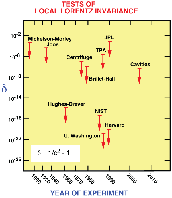
Figure 2: Selected tests of local Lorentz invariance showing the bounds on the parameter , which measures the degree of violation of Lorentz invariance in electromagnetism. The Michelson–Morley, Joos, Brillet–Hall and cavity experiments test the isotropy of the round-trip speed of light. The centrifuge, two-photon absorption (TPA) and JPL experiments test the isotropy of light speed using one-way propagation. The most precise experiments test isotropy of atomic energy levels. The limits assume a speed of Earth of relative to the mean rest frame of the universe.

The framework focuses exclusively on classical electrodynamics. It has recently been extended to the entire standard model of particle physics by Kostelecký and colleagues [92*, 93*, 228*]. The “standard model extension” (SME) has a large number of Lorentz-violating parameters, opening up many new opportunities for experimental tests (see Section 2.2.4). A variety of clock anisotropy experiments have been carried out to bound the electromagnetic parameters of the SME framework [227]. For example, the cavity experiments described above [438, 254, 293] placed bounds on the coefficients of the tensors and (see Section 2.2.4 for definitions) at the levels of and , respectively. Direct comparisons between atomic clocks based on different nuclear species place bounds on SME parameters in the neutron and proton sectors, depending on the nature of the transitions involved. The bounds achieved range from to . Recent examples include [440, 369].

Astrophysical observations have also been used to bound Lorentz violations. For example, if photons satisfy the Lorentz violating dispersion relation

where is the Planck energy, then the speed of light would be given, to linear order in the by Such a Lorentz-violating dispersion relation could be a relic of quantum gravity, for instance. By bounding the difference in arrival time of high-energy photons from a burst source at large distances, one could bound contributions to the dispersion for . One limit, comes from observations of 1 and 2 TeV gamma rays from the blazar Markarian 421 [48]. Another limit comes from birefringence in photon propagation: In many Lorentz violating models, different photon polarizations may propagate with different speeds, causing the plane of polarization of a wave to rotate. If the frequency dependence of this rotation has a dispersion relation similar to Eq. (3*), then by studying “polarization diffusion” of light from a polarized source in a given bandwidth, one can effectively place a bound  [173]. Measurements of the spectrum of ultra-high-energy cosmic rays using data from the HiRes and Pierre Auger observatories show no evidence for violations of Lorentz invariance [378, 47]. Other testable effects of Lorentz invariance violation include threshold effects in particle reactions, gravitational Cerenkov radiation, and neutrino oscillations.

For thorough and up-to-date surveys of both the theoretical frameworks and the experimental results for tests of LLI see the reviews by Mattingly [273*], Liberati [251*] and Kostelecký and Russell [229]. The last article gives “data tables” showing experimental bounds on all the various parameters of the SME.

Local Lorentz invariance can also be violated in gravitational interactions; these will be discussed under the rubric of “preferred-frame effects” in Section 4.3.2.

2.1.3 Tests of local position invariance

The principle of local position invariance, the third part of EEP, can be tested by the gravitational redshift experiment, the first experimental test of gravitation proposed by Einstein. Despite the fact that Einstein regarded this as a crucial test of GR, we now realize that it does not distinguish between GR and any other metric theory of gravity, but is only a test of EEP. The iconic gravitational redshift experiment measures the frequency or wavelength shift between two identical frequency standards (clocks) placed at rest at different heights in a static gravitational field. If the frequency of a given type of atomic clock is the same when measured in a local, momentarily co-moving freely falling frame (Lorentz frame), independent of the location or velocity of that frame, then the comparison of frequencies of two clocks at rest at different locations boils down to a comparison of the velocities of two local Lorentz frames, one at rest with respect to one clock at the moment of emission of its signal, the other at rest with respect to the other clock at the moment of reception of the signal. The frequency shift is then a consequence of the first-order Doppler shift between the frames. The structure of the clock plays no role whatsoever. The result is a shift

where is the difference in the Newtonian gravitational potential between the receiver and the emitter. If LPI is not valid, then it turns out that the shift can be written where the parameter may depend upon the nature of the clock whose shift is being measured (see TEGP 2.4 (c) [420*] for details).

The first successful, high-precision redshift measurement was the series of Pound–Rebka–Snider experiments of 1960 – 1965 that measured the frequency shift of gamma-ray photons from as they ascended or descended the Jefferson Physical Laboratory tower at Harvard University. The high accuracy achieved – one percent – was obtained by making use of the Mössbauer effect to produce a narrow resonance line whose shift could be accurately determined. Other experiments since 1960 measured the shift of spectral lines in the Sun’s gravitational field and the change in rate of atomic clocks transported aloft on aircraft, rockets and satellites. Figure 3* summarizes the important redshift experiments that have been performed since 1960 (TEGP 2.4 (c) [420*]).

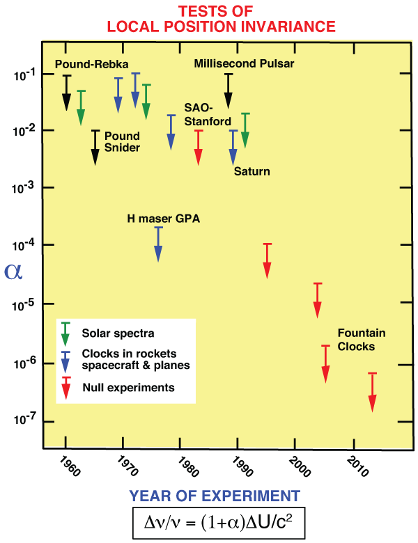
Figure 3: Selected tests of local position invariance via gravitational redshift experiments, showing bounds on , which measures degree of deviation of redshift from the formula . In null redshift experiments, the bound is on the difference in between different kinds of clocks.

After almost 50 years of inconclusive or contradictory measurements, the gravitational redshift of solar spectral lines was finally measured reliably. During the early years of GR, the failure to measure this effect in solar lines was seized upon by some as reason to doubt the theory (see [95*] for an engaging history of this period). Unfortunately, the measurement is not simple. Solar spectral lines are subject to the “limb effect”, a variation of spectral line wavelengths between the center of the solar disk and its edge or “limb”; this effect is actually a Doppler shift caused by complex convective and turbulent motions in the photosphere and lower chromosphere, and is expected to be minimized by observing at the solar limb, where the motions are predominantly transverse to the line of sight. The secret is to use strong, symmetrical lines, leading to unambiguous wavelength measurements. Successful measurements were finally made in 1962 and 1972 (TEGP 2.4 (c) [420*]). In 1991, LoPresto et al. [259] measured the solar shift in agreement with LPI to about 2 percent by observing the oxygen triplet lines both in absorption in the limb and in emission just off the limb.

The most precise standard redshift test to date was the Vessot–Levine rocket experiment known as Gravity Probe-A (GPA) that took place in June 1976 [400]. A hydrogen-maser clock was flown on a rocket to an altitude of about 10 000 km and its frequency compared to a hydrogen-maser clock on the ground. The experiment took advantage of the masers’ frequency stability by monitoring the frequency shift as a function of altitude. A sophisticated data acquisition scheme accurately eliminated all effects of the first-order Doppler shift due to the rocket’s motion, while tracking data were used to determine the payload’s location and the velocity (to evaluate the potential difference , and the special relativistic time dilation). Analysis of the data yielded a limit .

A “null” redshift experiment performed in 1978 tested whether the relative rates of two different clocks depended upon position. Two hydrogen maser clocks and an ensemble of three superconducting-cavity stabilized oscillator (SCSO) clocks were compared over a 10-day period. During the period of the experiment, the solar potential within the laboratory was known to change sinusoidally with a 24-hour period by because of the Earth’s rotation, and to change linearly at per day because the Earth is 90 degrees from perihelion in April. However, analysis of the data revealed no variations of either type within experimental errors, leading to a limit on the LPI violation parameter  [391]. This bound has been improved using more stable frequency standards, such as atomic fountain clocks [174, 326, 34, 63]. The best current bounds, from comparing a Rubidium atomic fountain with a Cesium-133 fountain or with a hydrogen maser [179, 319], and from comparing transitions of two different isotopes of Dysprosium [246], hover around the one part per million mark.

The Atomic Clock Ensemble in Space (ACES) project will place both a cold trapped atom clock based on Cesium called PHARAO (Projet d’Horloge Atomique par Refroidissement d’Atomes en Orbite), and an advanced hydrogen maser clock on the International Space Station to measure the gravitational redshift to parts in , as well as to carry out a number of fundamental physics experiments and to enable improvements in global timekeeping [335]. Launch is currently scheduled for May 2016.

The varying gravitational redshift of Earth-bound clocks relative to the highly stable millisecond pulsar PSR 1937+21, caused by the Earth’s motion in the solar gravitational field around the Earth-Moon center of mass (amplitude 4000 km), was measured to about 10 percent [383]. Two measurements of the redshift using stable oscillator clocks on spacecraft were made at the one percent level: one used the Voyager spacecraft in Saturn’s gravitational field [233], while another used the Galileo spacecraft in the Sun’s field [235].

The gravitational redshift could be improved to the level using an array of laser cooled atomic clocks on board a spacecraft which would travel to within four solar radii of the Sun [270]. Sadly, the Solar Probe Plus mission, scheduled for launch in 2018, has been formulated as an exclusively heliophysics mission, and thus will not be able to test fundamental gravitational physics.

Modern advances in navigation using Earth-orbiting atomic clocks and accurate time-transfer must routinely take gravitational redshift and time-dilation effects into account. For example, the Global Positioning System (GPS) provides absolute positional accuracies of around 15 m (even better in its military mode), and 50 nanoseconds in time transfer accuracy, anywhere on Earth. Yet the difference in rate between satellite and ground clocks as a result of relativistic effects is a whopping 39 microseconds per day ( from the gravitational redshift, and from time dilation). If these effects were not accurately accounted for, GPS would fail to function at its stated accuracy. This represents a welcome practical application of GR! (For the role of GR in GPS, see [25, 26]; for a popular essay, see [424].)

A final example of the almost “everyday” implications of the gravitational redshift is a remarkable measurement using optical clocks based on trapped aluminum ions of the frequency shift over a height of 1/3 of a meter [80].

Local position invariance also refers to position in time. If LPI is satisfied, the fundamental constants of non-gravitational physics should be constants in time. Table 1 shows current bounds on cosmological variations in selected dimensionless constants. For discussion and references to early work, see TEGP 2.4 (c) [420*] or [138]. For a comprehensive recent review both of experiments and of theoretical ideas that underlie proposals for varying constants, see [397].

Experimental bounds on varying constants come in two types: bounds on the present rate of variation, and bounds on the difference between today’s value and a value in the distant past. The main example of the former type is the clock comparison test, in which highly stable atomic clocks of different fundamental type are intercompared over periods ranging from months to years (variants of the null redshift experiment). If the frequencies of the clocks depend differently on the electromagnetic fine structure constant , the electron-proton mass ratio , or the gyromagnetic ratio of the proton , for example, then a limit on a drift of the fractional frequency difference translates into a limit on a drift of the constant(s). The dependence of the frequencies on the constants may be quite complex, depending on the atomic species involved. Experiments have exploited the techniques of laser cooling and trapping, and of atom fountains, in order to achieve extreme clock stability, and compared the Rubidium-87 hyperfine transition [271], the Mercury-199 ion electric quadrupole transition [49], the atomic Hydrogen transition [159], or an optical transition in Ytterbium-171 [318], against the ground-state hyperfine transition in Cesium-133. More recent experiments have used Strontium-87 atoms trapped in optical lattices [63] compared with Cesium to obtain , compared Rubidium-87 and Cesium-133 fountains [179] to obtain , or compared two isotopes of Dysprosium [246] to obtain ,.

The second type of bound involves measuring the relics of or signal from a process that occurred in the distant past and comparing the inferred value of the constant with the value measured in the laboratory today. One sub-type uses astronomical measurements of spectral lines at large redshift, while the other uses fossils of nuclear processes on Earth to infer values of constants early in geological history.

Earlier comparisons of spectral lines of different atoms or transitions in distant galaxies and quasars produced bounds or on the order of a part in 10 per Hubble time [441]. Dramatic improvements in the precision of astronomical and laboratory spectroscopy, in the ability to model the complex astronomical environments where emission and absorption lines are produced, and in the ability to reach large redshift have made it possible to improve the bounds significantly. In fact, in 1999, Webb et al. [406, 296] announced that measurements of absorption lines in Mg, Al, Si, Cr, Fe, Ni, and Zn in quasars in the redshift range indicated a smaller value of in earlier epochs, namely , corresponding to (assuming a linear drift with time). The Webb group continues to report changes in over large redshifts [217]. Measurements by other groups have so far failed to confirm this non-zero effect [373*, 76, 329]; an analysis of Mg absorption systems in quasars at gave  [373]. Recent studies have also yielded no evidence for a variation in  [210, 248]

Another important set of bounds arises from studies of the “Oklo” phenomenon, a group of natural, sustained fission reactors that occurred in the Oklo region of Gabon, Africa, around 1.8 billion years ago. Measurements of ore samples yielded an abnormally low value for the ratio of two isotopes of Samarium, . Neither of these isotopes is a fission product, but can be depleted by a flux of neutrons. Estimates of the neutron fluence (integrated dose) during the reactors’ “on” phase, combined with the measured abundance anomaly, yield a value for the neutron cross-section for 1.8 billion years ago that agrees with the modern value. However, the capture cross-section is extremely sensitive to the energy of a low-lying level (), so that a variation in the energy of this level of only 20 meV over a billion years would change the capture cross-section from its present value by more than the observed amount. This was first analyzed in 1976 by Shlyakter [365]. Recent reanalyses of the Oklo data [101, 166, 320] lead to a bound on at the level of around .

In a similar manner, recent reanalyses of decay rates of in ancient meteorites (4.5 billion years old) gave the bound  [312].

2.2 Theoretical frameworks for analyzing EEP

2.2.1 Schiff’s conjecture

Because the three parts of the Einstein equivalence principle discussed above are so very different in their empirical consequences, it is tempting to regard them as independent theoretical principles. On the other hand, any complete and self-consistent gravitation theory must possess sufficient mathematical machinery to make predictions for the outcomes of experiments that test each principle, and because there are limits to the number of ways that gravitation can be meshed with the special relativistic laws of physics, one might not be surprised if there were theoretical connections between the three sub-principles. For instance, the same mathematical formalism that produces equations describing the free fall of a hydrogen atom must also produce equations that determine the energy levels of hydrogen in a gravitational field, and thereby the ticking rate of a hydrogen maser clock. Hence a violation of EEP in the fundamental machinery of a theory that manifests itself as a violation of WEP might also be expected to show up as a violation of local position invariance. Around 1960, Leonard Schiff conjectured that this kind of connection was a necessary feature of any self-consistent theory of gravity. More precisely, Schiff’s conjecture states that any complete, self-consistent theory of gravity that embodies WEP necessarily embodies EEP. In other words, the validity of WEP alone guarantees the validity of local Lorentz and position invariance, and thereby of EEP.

If Schiff’s conjecture is correct, then Eötvös experiments may be seen as the direct empirical foundation for EEP, hence for the interpretation of gravity as a curved-spacetime phenomenon. Of course, a rigorous proof of such a conjecture is impossible (indeed, some special counter-examples are known [311, 300*, 91]), yet a number of powerful “plausibility” arguments can be formulated.

The most general and elegant of these arguments is based upon the assumption of energy conservation. This assumption allows one to perform very simple cyclic gedanken experiments in which the energy at the end of the cycle must equal that at the beginning of the cycle. This approach was pioneered by Dicke, Nordtvedt, and Haugan (see, e.g., [181*]). A system in a quantum state decays to state , emitting a quantum of frequency . The quantum falls a height in an external gravitational field and is shifted to frequency , while the system in state falls with acceleration . At the bottom, state is rebuilt out of state , the quantum of frequency , and the kinetic energy that state has gained during its fall. The energy left over must be exactly enough, , to raise state to its original location. (Here an assumption of local Lorentz invariance permits the inertial masses and to be identified with the total energies of the bodies.) If and depend on that portion of the internal energy of the states that was involved in the quantum transition from to according to

(violation of WEP), then by conservation of energy, there must be a corresponding violation of LPI in the frequency shift of the form (to lowest order in ) Haugan generalized this approach to include violations of LLI [181] (TEGP 2.5 [420*]).

2.2.2 The formalism

The first successful attempt to prove Schiff’s conjecture more formally was made by Lightman and Lee [252]. They developed a framework called the formalism that encompasses all metric theories of gravity and many non-metric theories (see Box 1). It restricts attention to the behavior of charged particles (electromagnetic interactions only) in an external static spherically symmetric (SSS) gravitational field, described by a potential . It characterizes the motion of the charged particles in the external potential by two arbitrary functions and , and characterizes the response of electromagnetic fields to the external potential (gravitationally modified Maxwell equations) by two functions and . The forms of , , , and vary from theory to theory, but every metric theory satisfies

for all . This consequence follows from the action of electrodynamics with a “minimal” or metric coupling: where the variables are defined in Box 1, and where . By identifying and in a SSS field, and , one obtains Eq. (9*). Conversely, every theory within this class that satisfies Eq. (9*) can have its electrodynamic equations cast into “metric” form. In a given non-metric theory, the functions , , , and will depend in general on the full gravitational environment, including the potential of the Earth, Sun, and Galaxy, as well as on cosmological boundary conditions. Which of these factors has the most influence on a given experiment will depend on the nature of the experiment.

Lightman and Lee then calculated explicitly the rate of fall of a “test” body made up of interacting charged particles, and found that the rate was independent of the internal electromagnetic structure of the body (WEP) if and only if Eq. (9*) was satisfied. In other words, WEP EEP and Schiff’s conjecture was verified, at least within the restrictions built into the formalism.

Certain combinations of the functions , , , and reflect different aspects of EEP. For instance, position or -dependence of either of the combinations and signals violations of LPI, the first combination playing the role of the locally measured electric charge or fine structure constant. The “non-metric parameters” and (see Box 1) are measures of such violations of EEP. Similarly, if the parameter is non-zero anywhere, then violations of LLI will occur. This parameter is related to the difference between the speed of light , and the limiting speed of material test particles , given by

In many applications, by suitable definition of units, can be set equal to unity. If EEP is valid, everywhere.

The rate of fall of a composite spherical test body of electromagnetically interacting particles then has the form

where and are the electrostatic and magnetostatic binding energies of the body, given by where , , and the angle brackets denote an expectation value of the enclosed operator for the system’s internal state. Eötvös experiments place limits on the WEP-violating terms in Eq. (13*), and ultimately place limits on the non-metric parameters and . (We set because of very tight constraints on it from tests of LLI; see Figure 2*, where .) These limits are sufficiently tight to rule out a number of non-metric theories of gravity thought previously to be viable (TEGP 2.6 (f) [420*]).

The formalism also yields a gravitationally modified Dirac equation that can be used to determine the gravitational redshift experienced by a variety of atomic clocks. For the redshift parameter (see Eq. (6*)), the results are (TEGP 2.6 (c) [420*]):

The redshift is the standard one , independently of the nature of the clock if and only if . Thus the Vessot–Levine rocket redshift experiment sets a limit on the parameter combination (see Figure 3*); the null-redshift experiment comparing hydrogen-maser and SCSO clocks sets a limit on . Alvarez and Mann [9, 10, 11, 12, 13] extended the formalism to permit analysis of such effects as the Lamb shift, anomalous magnetic moments and non-baryonic effects, and placed interesting bounds on EEP violations.

2.2.3 The formalism

The formalism can also be applied to tests of local Lorentz invariance, but in this context it can be simplified. Since most such tests do not concern themselves with the spatial variation of the functions , , , and , but rather with observations made in moving frames, we can treat them as spatial constants. Then by rescaling the time and space coordinates, the charges and the electromagnetic fields, we can put the action in Box 1 into the form (TEGP 2.6 (a) [420*])

where . This amounts to using units in which the limiting speed of massive test particles is unity, and the speed of light is . If , LLI is violated; furthermore, the form of the action above must be assumed to be valid only in some preferred universal rest frame. The natural candidate for such a frame is the rest frame of the microwave background.

The electrodynamical equations which follow from Eq. (17*) yield the behavior of rods and clocks, just as in the full formalism. For example, the length of a rod which moves with velocity relative to the rest frame in a direction parallel to its length will be observed by a rest observer to be contracted relative to an identical rod perpendicular to the motion by a factor . Notice that does not appear in this expression, because only electrostatic interactions are involved, and appears only in the magnetic sector of the action (17*). The energy and momentum of an electromagnetically bound body moving with velocity relative to the rest frame are given by

where , is the sum of the particle rest masses, is the electrostatic binding energy of the system (see Eq. (14*) with ), and where Note that corresponds to the parameter plotted in Figure 2*.

The electrodynamics given by Eq. (17*) can also be quantized, so that we may treat the interaction of photons with atoms via perturbation theory. The energy of a photon is times its frequency , while its momentum is . Using this approach, one finds that the difference in round trip travel times of light along the two arms of the interferometer in the Michelson–Morley experiment is given by . The experimental null result then leads to the bound on shown on Figure 2*. Similarly the anisotropy in energy levels is clearly illustrated by the tensorial terms in Eqs. (18*, 20*); by evaluating for each nucleus in the various Hughes–Drever-type experiments and comparing with the experimental limits on energy differences, one obtains the extremely tight bounds also shown on Figure 2*.

The behavior of moving atomic clocks can also be analyzed in detail, and bounds on can be placed using results from tests of time dilation and of the propagation of light. In some cases, it is advantageous to combine the framework with a “kinematical” viewpoint that treats a general class of boost transformations between moving frames. Such kinematical approaches have been discussed by Robertson, Mansouri and Sexl, and Will (see [418*]).

For example, in the “JPL” experiment, in which the phases of two hydrogen masers connected by a fiberoptic link were compared as a function of the Earth’s orientation, the predicted phase difference as a function of direction is, to first order in , the velocity of the Earth through the cosmic background,

where , is the maser frequency, is the baseline, and where and are unit vectors along the direction of propagation of the light at a given time and at the initial time of the experiment, respectively. The observed limit on a diurnal variation in the relative phase resulted in the bound . Tighter bounds were obtained from a “two-photon absorption” (TPA) experiment, and a 1960s series of “Mössbauer-rotor” experiments, which tested the isotropy of time dilation between a gamma ray emitter on the rim of a rotating disk and an absorber placed at the center [418].

2.2.4 The standard model extension (SME)

Kostelecký and collaborators developed a useful and elegant framework for discussing violations of Lorentz symmetry in the context of the standard model of particle physics [92, 93, 228]. Called the standard model extension (SME), it takes the standard field theory of particle physics, and modifies the terms in the action by inserting a variety of tensorial quantities in the quark, lepton, Higgs, and gauge boson sectors that could explicitly violate LLI. SME extends the earlier classical and frameworks, and the framework of Ni [300] to quantum field theory and particle physics. The modified terms split naturally into those that are odd under CPT (i.e., that violate CPT) and terms that are even under CPT. The result is a rich and complex framework, with many parameters to be analyzed and tested by experiment. Such details are beyond the scope of this review; for a review of SME and other frameworks, the reader is referred to the Living Review by Mattingly [273] or the review by Liberati [251]. The review of the SME by Kostelecký and Russell [229] provides “data tables” showing experimental bounds on all the various parameters of the SME.

Here we confine our attention to the electromagnetic sector, in order to link the SME with the framework discussed above. In the SME, the Lagrangian for a scalar particle with charge interacting with electrodynamics takes the form

where , where is a real symmetric trace-free tensor, and where is a tensor with the symmetries of the Riemann tensor, and with vanishing double trace. It has 19 independent components. There could also be a CPT-odd term in of the form , but because of a variety of pre-existing theoretical and experimental constraints, it is generally set to zero.

The tensor can be decomposed into “electric”, “magnetic”, and “odd-parity” components, by defining

In many applications it is useful to use the further decomposition The first expression is a single number, the next three are symmetric trace-free matrices, and the final is an antisymmetric matrix, accounting thereby for the 19 components of the original tensor .

In the rest frame of the universe, these tensors have some form that is established by the global nature of the solutions of the overarching theory being used. In a frame that is moving relative to the universe, the tensors will have components that depend on the velocity of the frame, and on the orientation of the frame relative to that velocity.

In the case where the theory is rotationally symmetric in the preferred frame, the tensors and can be expressed in the form

where around indices denote antisymmetrization, and where is the four-velocity of an observer at rest in the preferred frame. With this assumption, all the tensorial quantities in Eq. (24*) vanish in the preferred frame, and, after suitable rescalings of coordinates and fields, the action (22*) can be put into the form of the framework, with

2.3 EEP, particle physics, and the search for new interactions

Thus far, we have discussed EEP as a principle that strictly divides the world into metric and non-metric theories, and have implied that a failure of EEP might invalidate metric theories (and thus general relativity). On the other hand, there is mounting theoretical evidence to suggest that EEP is likely to be violated at some level, whether by quantum gravity effects, by effects arising from string theory, or by hitherto undetected interactions. Roughly speaking, in addition to the pure Einsteinian gravitational interaction, which respects EEP, theories such as string theory predict other interactions which do not. In string theory, for example, the existence of such EEP-violating fields is assured, but the theory is not yet mature enough to enable a robust calculation of their strength relative to gravity, or a determination of whether they are long range, like gravity, or short range, like the nuclear and weak interactions, and thus too short-range to be detectable.

In one simple example [129], one can write the Lagrangian for the low-energy limit of a string-inspired theory in the so-called “Einstein frame”, in which the gravitational Lagrangian is purely general relativistic:

where is the non-physical metric, is the Ricci tensor derived from it, is a dilaton field, and , and are functions of . The Lagrangian includes that for the electromagnetic field , and that for particles, written in terms of Dirac spinors . This is not a metric representation because of the coupling of to matter via and . A conformal transformation , , puts the Lagrangian in the form (“Jordan” frame) One may choose so that the particle Lagrangian takes the metric form (no explicit coupling to ), but the electromagnetic Lagrangian will still couple non-metrically to . The gravitational Lagrangian here takes the form of a scalar–tensor theory (see Section 3.3.2). But the non-metric electromagnetic term will, in general, produce violations of EEP. For examples of specific models, see [384*, 117*]. Another class of non-metric theories is the “varying speed of light (VSL)” set of theories; for a detailed review, see [268].

On the other hand, whether one views such effects as a violation of EEP or as effects arising from additional “matter” fields whose interactions, like those of the electromagnetic field, do not fully embody EEP, is to some degree a matter of semantics. Unlike the fields of the standard model of electromagnetic, weak and strong interactions, which couple to properties other than mass-energy and are either short range or are strongly screened, the fields inspired by string theory could be long range (if they remain massless by virtue of a symmetry, or at best, acquire a very small mass), and can couple to mass-energy, and thus can mimic gravitational fields. Still, there appears to be no way to make this precise.

As a result, EEP and related tests are now viewed as ways to discover or place constraints on new physical interactions, or as a branch of “non-accelerator particle physics”, searching for the possible imprints of high-energy particle effects in the low-energy realm of gravity. Whether current or proposed experiments can actually probe these phenomena meaningfully is an open question at the moment, largely because of a dearth of firm theoretical predictions.

2.3.1 The “fifth” force

On the phenomenological side, the idea of using EEP tests in this way may have originated in the middle 1980s, with the search for a “fifth” force. In 1986, as a result of a detailed reanalysis of Eötvös’ original data, Fischbach et al. [156] suggested the existence of a fifth force of nature, with a strength of about a percent that of gravity, but with a range (as defined by the range of a Yukawa potential, ) of a few hundred meters. This proposal dovetailed with earlier hints of a deviation from the inverse-square law of Newtonian gravitation derived from measurements of the gravity profile down deep mines in Australia, and with emerging ideas from particle physics suggesting the possible presence of very low-mass particles with gravitational-strength couplings. During the next four years numerous experiments looked for evidence of the fifth force by searching for composition-dependent differences in acceleration, with variants of the Eötvös experiment or with free-fall Galileo-type experiments. Although two early experiments reported positive evidence, the others all yielded null results. Over the range between one and meters, the null experiments produced upper limits on the strength of a postulated fifth force between and of the strength of gravity. Interpreted as tests of WEP (corresponding to the limit of infinite-range forces), the results of two representative experiments from this period, the free-fall Galileo experiment and the early Eöt-Wash experiment, are shown in Figure 1*. At the same time, tests of the inverse-square law of gravity were carried out by comparing variations in gravity measurements up tall towers or down mines or boreholes with gravity variations predicted using the inverse square law together with Earth models and surface gravity data mathematically “continued” up the tower or down the hole. Despite early reports of anomalies, independent tower, borehole, and seawater measurements ultimately showed no evidence of a deviation. Analyses of orbital data from planetary range measurements, lunar laser ranging (LLR), and laser tracking of the LAGEOS satellite verified the inverse-square law to parts in over scales of to , and to parts in over planetary scales of several astronomical units [381*]. A consensus emerged that there was no credible experimental evidence for a fifth force of nature, of a type and range proposed by Fischbach et al. For reviews and bibliographies of this episode, see [155, 157, 158, 4, 417].

2.3.2 Short-range modifications of Newtonian gravity

Although the idea of an intermediate-range violation of Newton’s gravitational law was dropped, new ideas emerged to suggest the possibility that the inverse-square law could be violated at very short ranges, below the centimeter range of existing laboratory verifications of the behavior. One set of ideas [18, 21, 331, 330] posited that some of the extra spatial dimensions that come with string theory could extend over macroscopic scales, rather than being rolled up at the Planck scale of , which was then the conventional viewpoint. On laboratory distances large compared to the relevant scale of the extra dimension, gravity would fall off as the inverse square, whereas on short scales, gravity would fall off as , where is the number of large extra dimensions. Many models favored or . Other possibilities for effective modifications of gravity at short range involved the exchange of light scalar particles.

Following these proposals, many of the high-precision, low-noise methods that were developed for tests of WEP were adapted to carry out laboratory tests of the inverse square law of Newtonian gravitation at millimeter scales and below. The challenge of these experiments has been to distinguish gravitation-like interactions from electromagnetic and quantum mechanical (Casimir) effects. No deviations from the inverse square law have been found to date at distances between tens of nanometers and 10 mm [258, 193, 192, 79, 257, 211, 2, 390, 172, 380, 45, 449, 218]. For a comprehensive review of both the theory and the experiments circa 2002, see [3].

2.3.3 The Pioneer anomaly

In 1998, Anderson et al. [16] reported the presence of an anomalous deceleration in the motion of the Pioneer 10 and 11 spacecraft at distances between 20 and 70 astronomical units from the Sun. Although the anomaly was the result of a rigorous analysis of Doppler data taken over many years, it might have been dismissed as having no real significance for new physics, where it not for the fact that the acceleration, of order , when divided by the speed of light, was strangely close to the inverse of the Hubble time. The Pioneer anomaly prompted an outpouring of hundreds of papers, most attempting to explain it via modifications of gravity or via new physical interactions, with a small subset trying to explain it by conventional means.

Soon after the publication of the initial Pioneer anomaly paper [16], Katz pointed out that the anomaly could be accounted for as the result of the anisotropic emission of radiation from the radioactive thermal generators (RTG) that continued to power the spacecraft decades after their launch [212]. At the time, there was insufficient data on the performance of the RTG over time or on the thermal characteristics of the spacecraft to justify more than an order-of-magnitude estimate. However, the recovery of an extended set of Doppler data covering a longer stretch of the orbits of both spacecraft, together with the fortuitous discovery of project documentation and of telemetry data giving on-board temperature information, made it possible both to improve the orbit analysis and to develop detailed thermal models of the spacecraft in order to quantify the effect of thermal emission anisotropies. Several independent analyses now confirm that the anomaly is almost entirely due to the recoil of the spacecraft from the anisotropic emission of residual thermal radiation [339, 396, 291]. For a thorough review of the Pioneer anomaly published just as the new analyses were underway, see the Living Review by Turyshev and Toth [395].