 -decoupling
limit of bi-gravity
-decoupling
limit of bi-gravity
 )
)5 Deconstruction
As for DGP and its extensions, to get some insight on how to construct a four-dimensional theory of single massive graviton, we can start with five-dimensional general relativity. This time, we consider the extra dimension to be compactified and of finite size , with periodic boundary conditions. It is then
natural to perform a Kaluza–Klein decomposition and to obtain a tower of Kaluza–Klein graviton mode in
four dimensions. The zero mode is then massless and the higher modes are all massive with mass separation
, with periodic boundary conditions. It is then
natural to perform a Kaluza–Klein decomposition and to obtain a tower of Kaluza–Klein graviton mode in
four dimensions. The zero mode is then massless and the higher modes are all massive with mass separation
 . Since the graviton mass is constant in this formalism we omit the subscript
  in the rest of
this review.
in the rest of
this review.
Rather than starting directly with a Kaluza–Klein decomposition (discretization in Fourier space), we perform instead a discretization in real space, known as “deconstruction” of five-dimensional gravity [24*, 25*, 170*, 168*, 28*, 443*, 340*]. The deconstruction framework helps making the connection with massive gravity more explicit. However, we can also obtain multi-gravity out of it which is then completely equivalent to the Kaluza–Klein decomposition (after a non-linear field redefinition).
The idea behind deconstruction is simply to ‘replace’ the continuous fifth dimension  by a series of
 sites
sites  separated by a distance
  . So that the five-dimensional metric is replaced by a set
of
. So that the five-dimensional metric is replaced by a set
of  interacting metrics depending only on
  .
.
In what follows, we review the procedure derived in [152*] to recover four-dimensional ghost-free massive gravity as well as bi- and multi-gravity out of five-dimensional GR. The procedure works in any dimensions and we only focus to deconstructing five-dimensional GR for sake of concreteness.
5.1 Formalism
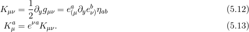
5.1.1 Metric versus Einstein–Cartan formulation of GR
Before going further, let us first describe five-dimensional general relativity in its Einstein–Cartan
formulation, where we introduce a set of vielbein  , so that the relation between the metric and the
vielbein is simply,
, so that the relation between the metric and the
vielbein is simply,

 label five-dimensional Lorentz indices.
Under the torsionless condition,  , the antisymmetric spin connection
  , is uniquely
determined in terms of the vielbeins
, is uniquely
determined in terms of the vielbeins

![ab aA bB O c = 2e e ∂ [AeB ]c](article677x.gif) . In the Einstein–Cartan formulation of GR, we introduce a 2-form Riemann
curvature,
and up to boundary terms, the Einstein–Hilbert action is then given in the respective metric and the
vielbein languages by (here in five dimensions for definiteness),
where
. In the Einstein–Cartan formulation of GR, we introduce a 2-form Riemann
curvature,
and up to boundary terms, the Einstein–Hilbert action is then given in the respective metric and the
vielbein languages by (here in five dimensions for definiteness),
where 
![M 3 ∫ √ --- SE(5H)= --5- d4x dy − gR (5)[g] (5.4 ) 2 ∫ M 53 ab c d e = ------ 𝜀abcdeℛ ∧ e ∧ e ∧ e , (5.5 ) 2 × 3!](article679x.gif)
![R(5)[g]](article680x.gif) is the scalar curvature built out of the five-dimensional metric
is the scalar curvature built out of the five-dimensional metric  and
and  is the
five-dimensional Planck scale.
is the
five-dimensional Planck scale.
The counting of the degrees of freedom in both languages is of course equivalent and goes as follows: In
 -spacetime dimensions, the metric has
  independent components. Covariance removes
  of
them,10
which leads to
of
them,10
which leads to  independent degrees of freedom. In four-dimensions, we recover the usual
 independent polarizations for gravitational waves. In five-dimensions, this leads to
  degrees of freedom which is the same number of degrees of freedom as a massive spin-2 field in four
dimensions. This is as expect from the Kaluza–Klein philosophy (massless bosons in
degrees of freedom which is the same number of degrees of freedom as a massive spin-2 field in four
dimensions. This is as expect from the Kaluza–Klein philosophy (massless bosons in  dimensions
have the same number of degrees of freedom as massive bosons in
dimensions
have the same number of degrees of freedom as massive bosons in  dimensions – this counting does not
directly apply to fermions).
dimensions – this counting does not
directly apply to fermions).
In the Einstein–Cartan formulation, the counting goes as follows: The vielbein has  independent
components. Covariance removes
independent
components. Covariance removes  of them, and the additional global Lorentz invariance removes an
additional
of them, and the additional global Lorentz invariance removes an
additional  , leading once again to a total of
  independent degrees of
freedom.
independent degrees of
freedom.
In GR one usually considers the metric and the vielbein formulation as being fully equivalent. However,
this perspective is true only in the bosonic sector. The limitations of the metric formulation becomes
manifest when coupling gravity to fermions. For such couplings one requires the vielbein formulation of GR.
For instance, in four spacetime dimensions, the covariant action for a Dirac fermion  at the quadratic
order is given by (see Ref. [392]),
at the quadratic
order is given by (see Ref. [392]),
![∫ 1 [ i ←→ m ] SDirac = --𝜀abcd ea ∧ eb ∧ ec -¯ψ γdD ψ − --edψ¯ψ , (5.6 ) 3! 2 4](article699x.gif)
 ’s are the Dirac matrices and
  represents the covariant derivative,
![D ψ = dψ − 1ωab [γ ,γ ]ψ 8 a b](article702x.gif) .
.
In the bosonic sector, one can convert the covariant action of bosonic fields (e.g., of scalar, vector fields, etc…) between the vielbein and the metric language without much confusion, however this is not possible for the covariant Dirac action, or other half-spin fields. For these types of matter fields, the Einstein–Cartan Formulation of GR is more fundamental than its metric formulation. In doubt, one should always start with the vielbein formulation. This is especially important in the case of deconstruction when a discretization in the metric language is not equivalent to a discretization in the vielbein variables. The same holds for Kaluza–Klein decomposition, a point which might have been under-appreciated in the past.
5.1.2 Gauge-fixing
The discretization process breaks covariance and so before staring this procedure it is wise to fix the gauge (failure to do so leads to spurious degrees of freedom which then become ghost in the four-dimensional description). We thus start in five spacetime dimensions by setting the gauge
meaning that the lapse is set to unity and the shift to zero. Notice that one could in principle only set the lapse to unity and keep the shift present throughout the discretization. From a four-dimensional point of view, the shift will then ‘morally’ play the role of the Stückelberg fields, however they do so only after a cumbersome field redefinition. So for sake of clarity and simplicity, in what follows we first gauge-fix the shift and then once the four-dimensional theory is obtained to restore gauge invariance by use of the Stückelberg trick presented previously.
In vielbein language, we fix the five-dimensional coordinate system and use four Lorentz transformations to set
and use the remaining six Lorentz transformations to set
![ab μ[a b] ωy = e ∂yeμ = 0. (5.9 )](article705x.gif)
In this gauge, the five-dimensional Einstein–Hilbert term (5.4*), (5.5*) is given by
where![∫ (5) M 35 4 √ ---( 2 2) SEH = ---- d x dy − g R [g] + [K ] − [K ] (5.10 ) 23 ∫ ( = M-5- 𝜀 Rab ∧ ec ∧ ed − Ka ∧ Kb ∧ ec ∧ ed (5.11 ) 4 abcd a b c d) +2K ∧ ∂ye ∧ e ∧ e ∧ dy,](article706x.gif)
![R[g]](article707x.gif) , is the four-dimensional curvature built out of the four-dimensional metric
, is the four-dimensional curvature built out of the four-dimensional metric  ,
,
 is the 2-form curvature built out of the four-dimensional vielbein
  and its associated
connection
and its associated
connection  ,
,  , and
, and  is the extrinsic curvature,
5.1.3 Discretization in the vielbein
One could in principle go ahead and perform the discretization directly at the level of the metric but first this would not lead to a consistent truncated theory of massive gravity.11 As explained previously, the vielbein is more fundamental than the metric itself, and in what follows we discretize the theory keeping the vielbein as the fundamental object.
The gauge choice (5.9*) then implies where the arrow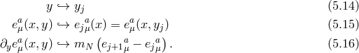
![ωayb= eμ[a∂yebμ]= 0 `→ ej+1μ[aejbμ]= 0, (5.17 )](article716x.gif)
 represents the deconstruction of five-dimensional gravity. We have also introduced the
‘truncation scale’,
represents the deconstruction of five-dimensional gravity. We have also introduced the
‘truncation scale’,  , i.e., the scale of the highest mode in the discretized
theory. After discretization, we see the Deser–van Nieuwenhuizen [187] condition appearing in
Eq. (5.17*), which corresponds to the symmetric vielbein condition. This is a sufficient condition to
allow for a formulation back into the metric language [410*, 314*, 172]. Note, however, that as
mentioned in [152*], we have not assumed that this symmetric vielbein condition was true,
we simply derived it from the discretization procedure in the five-dimensional gauge choice
, i.e., the scale of the highest mode in the discretized
theory. After discretization, we see the Deser–van Nieuwenhuizen [187] condition appearing in
Eq. (5.17*), which corresponds to the symmetric vielbein condition. This is a sufficient condition to
allow for a formulation back into the metric language [410*, 314*, 172]. Note, however, that as
mentioned in [152*], we have not assumed that this symmetric vielbein condition was true,
we simply derived it from the discretization procedure in the five-dimensional gauge choice
 .
.
In terms of the extrinsic curvature, this implies
This can be written back in the metric language as follows where the square root in the extrinsic curvature appears after converting back to the metric language. The square root exists as long as the metrics
![gμν(x,y ) `→ gj,μν(x ) = g μν(x, yj) (5.19 ) ( ( ∘ -------) μ) K μν `→ − mN 𝒦μν[gj,gj+1] ≡ − mN δμν − g−j1gj+1 , (5.20 ) ν](article721x.gif)
 and
and  have the same signature and
  has
positive eigenvalues so if both metrics were diagonal the ‘time’ direction associated with each metric would
be the same, which is a meaningful requirement.
has
positive eigenvalues so if both metrics were diagonal the ‘time’ direction associated with each metric would
be the same, which is a meaningful requirement.
From the metric language, we thus see that the discretization procedure amounts to converting
the extrinsic curvature to an interaction between neighboring sites through the building block
![𝒦 μ[g ,g ] ν j j+1](article725x.gif) .
.
5.2 Ghost-free massive gravity
5.2.1 Simplest discretization
In this subsection we focus on deriving a consistent theory of massive gravity from the discretization
procedure (5.19*, 5.20*). For this, we consider a discretization with only two sites  and will only be
considered in the four-dimensional action induced on one site (say site 1), rather than the sum of both sites.
This picture is analogous in spirit to a braneworld picture where we induce the action at one
point along the extra dimension. This picture gives the theory of a unique dynamical metric,
expressed in terms of a reference metric which corresponds to the fixed metric on the other site. We
emphasize that this picture corresponds to a trick to build a consistent theory of massive gravity,
and would otherwise be more artificial than its multi-gravity extension. However, as we shall
see later, massive gravity can be seen as a perfectly consistent limit of multi (or bi-)gravity
where the massless spin-2 field (and other fields in the multi-case) decouple and is thus perfectly
acceptable.
and will only be
considered in the four-dimensional action induced on one site (say site 1), rather than the sum of both sites.
This picture is analogous in spirit to a braneworld picture where we induce the action at one
point along the extra dimension. This picture gives the theory of a unique dynamical metric,
expressed in terms of a reference metric which corresponds to the fixed metric on the other site. We
emphasize that this picture corresponds to a trick to build a consistent theory of massive gravity,
and would otherwise be more artificial than its multi-gravity extension. However, as we shall
see later, massive gravity can be seen as a perfectly consistent limit of multi (or bi-)gravity
where the massless spin-2 field (and other fields in the multi-case) decouple and is thus perfectly
acceptable.
To simplify the notation for this two-site case, we write the vielbein on both sites as  ,
,  ,
and similarly for the metrics
,
and similarly for the metrics  and
and  . Out of the five-dimensional action for GR, we
obtain the theory of massive gravity in four dimensions, (on site 1),
. Out of the five-dimensional action for GR, we
obtain the theory of massive gravity in four dimensions, (on site 1),

![M 2 ∫ √ ---( ( )) S(m4G)R = --Pl d4x − g R [g] + m2 [𝒦 ]2 − [𝒦2 ] (5.22 ) 2 ∫ M P2l ( ab c d 2 abcd ) = --4- 𝜀abcd R ∧ e ∧ e + m 𝒜 (e,f) , (5.23 )](article732x.gif)


 , where in this case we limit the
integral about one site.
, where in this case we limit the
integral about one site.
The theory of massive gravity (5.22*), or equivalently (5.23*) is one special example of a ghost-free theory
of massive gravity (i.e., for which the BD ghost is absent). In terms of the ‘Stückelbergized’ tensor  introduced in Eq. (2.76*), we see that


![m2M 2Pl√ ---( 2 2) ℒmass = − ---2--- − g [𝒦 ] − [𝒦] (5.28 ) 2 2 ---( √ -- √ -- ) = − m--M-Pl√ − g [(𝕀 − 𝕏)2] − [𝕀 − 𝕏]2 . (5.29 ) 2](article739x.gif)
5.2.2 Generalized mass term
This mass term is not the unique acceptable generalization of Fierz–Pauli gravity and by considering more general discretization procedures we can generate the entire 2-parameter family of acceptable potentials for gravity which will also be shown to be free of ghost in Section 7.
Rather than considering the straight-forward discretization  , we could consider the
average value on one site, pondered with arbitrary weight
, we could consider the
average value on one site, pondered with arbitrary weight  ,
,


 is
thus12
with
for any
is
thus12
with
for any 

 .
.
In particular for the two-site case, this generates the two-parameter family of mass terms
with
 ,
,  ,
,  ,
,  and
and  . This corresponds to the most general potential which, by construction, includes no
cosmological constant nor tadpole. One can also always include a cosmological constant for
such models, which would naturally arise from a cosmological constant in the five-dimensional
picture.
. This corresponds to the most general potential which, by construction, includes no
cosmological constant nor tadpole. One can also always include a cosmological constant for
such models, which would naturally arise from a cosmological constant in the five-dimensional
picture.
We see that in the vielbein language, the expression for the mass term is extremely natural and simple. In fact this form was guessed at already for special cases in Ref. [410*] and even earlier in [502*]. However, the crucial analysis on the absence of ghosts and the reason for these terms was incorrect in both of these presentations. Subsequently, after the development of the consistent metric formulation, the generic form of the mass terms was given in Refs. [95*]13 and [314*].
In the metric Language, this corresponds to the following Lagrangian for dRGT massive gravity [144*], or its generalization to arbitrary reference metric [296*]
where the two parameters![∫ ( ) M 2Pl 4 √--- m2 ℒmGR = ---- d x − g R + --- (ℒ2 [𝒦] + α3ℒ3 [𝒦 ] + α4 ℒ4[𝒦 ]) , (5.35 ) 2 2](article754x.gif)
 are related to the two discretization parameters
  as
and for any tensor
as
and for any tensor 
 , we define the scalar
  symbolically as
for any
symbolically as
for any ![ℒn[Q ] = 𝜀𝜀Qn, (5.37 )](article760x.gif)
 , where
  is the number of spacetime dimensions.
  is the Levi-Cevita
antisymmetric symbol, so for instance in four dimensions,
is the Levi-Cevita
antisymmetric symbol, so for instance in four dimensions, ![′ ′ ℒ2 [Q ] = 𝜀μναβ𝜀μ′ν′αβQ μμ Q νν = 2!([Q]2 − [Q2 ])](article764x.gif) , so
we recover the mass term expressed in (5.28*). Their explicit form is given in what follows in the relations
(6.11*) – (6.13*) or (6.16*) – (6.18*).
, so
we recover the mass term expressed in (5.28*). Their explicit form is given in what follows in the relations
(6.11*) – (6.13*) or (6.16*) – (6.18*).
This procedure is easily generalizable to any number of dimensions, and massive gravity in
 dimensions has
  -free parameters which are related to the
  discretization
parameters.
discretization
parameters.
5.3 Multi-gravity
In Section 5.2, we showed how to obtain massive gravity from considering the five-dimensional Einstein–Hilbert action on
one site.14
Instead in this section, we integrate over the whole of the extra dimension, which corresponds to summing
over all the sites after discretization. Following the procedure of [152], we consider  sites to start which leads to multi-gravity [314*], and then focus on the two-site case leading to
bi-gravity [293*].
sites to start which leads to multi-gravity [314*], and then focus on the two-site case leading to
bi-gravity [293*].
Starting with the five-dimensional action (5.12*) and applying the discretization procedure (5.31*) with
 given in (5.33*), we get
![N ∫ M-42∑ ( ab c d 2 abcd ) SNmGR = 4 𝜀abcd R [ej] ∧ ej ∧ ej + m N𝒜 rj,sj(ej,ej+1) (5.38 ) j=1 ( ) M 2∑N ∫ ∘ ---- m2 ∑ 4 = --4- d4x − gj R [gj] +--N- α (jn)ℒn(𝒦j,j+1) , 2 j=1 2 n=0](article770x.gif)
 ,
,  , and in this deconstruction framework we obtain no
cosmological constant nor tadpole,
, and in this deconstruction framework we obtain no
cosmological constant nor tadpole,  at any site
  , (but we keep them for generality). In
the mass Lagrangian, we use the shorthand notation
, (but we keep them for generality). In
the mass Lagrangian, we use the shorthand notation  for the tensor
 ![𝒦 μ[g ,g ] ν j j+1](article776x.gif) . This is a special
case of multi-gravity presented in [314*] (see also [417] for other ‘topologies’ in the way the multiple
gravitons interact), where each metric only interacts with two other metrics, i.e., with its closest
neighbors, leading to
. This is a special
case of multi-gravity presented in [314*] (see also [417] for other ‘topologies’ in the way the multiple
gravitons interact), where each metric only interacts with two other metrics, i.e., with its closest
neighbors, leading to  -free parameters. For any fixed
  , one has
 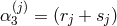 , and
, and
 .
.
To see the mass spectrum of this multi-gravity theory, we perform a Fourier decomposition, which is what one would obtain (after a field redefinition) by performing a KK decomposition rather than a real space discretization. KK decomposition and deconstruction are thus perfectly equivalent (after a non-linear – but benign15 – field redefinition). We define the discrete Fourier transform of the vielbein variables,
with the inverse map, In terms of the Fourier transform variables, the multi-gravity action then reads at the linear level with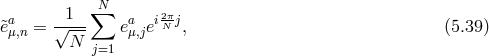
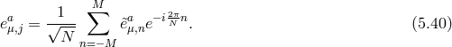
![∑M [ ] ℒ = (∂&tidle;hn )(∂ &tidle;h−n) + m2 &tidle;hn&tidle;h −n + ℒint (5.41 ) n= −M n](article783x.gif)
 and
and  represents the four-dimensional Planck scale,
 . The reality condition on the vielbein imposes
  and similarly for
  . The
mass spectrum is then
. The
mass spectrum is then

The counting of the degrees of freedom in multi-gravity goes as follows: the theory contains  massive spin-2 fields with five degrees of freedom each and one massless spin-2 field with two degrees of
freedom, corresponding to a total of
massive spin-2 fields with five degrees of freedom each and one massless spin-2 field with two degrees of
freedom, corresponding to a total of  degrees of freedom. In the continuum limit, we also need
to account for the zero mode of the lapse and the shift which have been gauged fixed in five
dimensions (see Ref. [443*] for a nice discussion of this point). This leads to three additional
degrees of freedom, summing up to a total of
degrees of freedom. In the continuum limit, we also need
to account for the zero mode of the lapse and the shift which have been gauged fixed in five
dimensions (see Ref. [443*] for a nice discussion of this point). This leads to three additional
degrees of freedom, summing up to a total of  degrees of freedom of the four coordinates
 .
.
5.4 Bi-gravity
Let us end this section with the special case of bi-gravity. Bi-gravity can also be derived from the deconstruction paradigm, just as massive gravity and multi-gravity, but the idea has been investigated for many years (see for instance [436, 324]). Like massive gravity, bi-gravity was for a long time thought to host a BD ghost parasite, but a ghost-free realization was recently proposed by Hassan and Rosen [293*] and bi-gravity is thus experiencing a revived amount of interested. This extensions is nothing other than the ghost-free massive gravity Lagrangian for a dynamical reference metric with the addition of an Einstein–Hilbert term for the now dynamical reference metric.
Bi-gravity from deconstruction
Let us consider a two-site discretization with periodic boundary conditions,  with quantities at
the site
with quantities at
the site  being identified with that at the site
  . Similarly, as in Section 5.2 we denote by
 and by
  ƒ
ƒ ƒ
ƒ the metrics and vielbeins at the respective locations
  and
and
 .
.
Then applying the discretization procedure highlighted in Eqs. (5.14*, 5.15*, 5.18*, 5.19* and 5.20*) and summing over the extra dimension, we obtain the bi-gravity action
where![2 ∫ --- M 2∫ ∘ ---- Sbi−gravity = M-Pl d4x√ − gR [g ] +--f- d4x − fR [f ] (5.43 ) 2 2 2 2 ∫ √ ---∑ 4 + M-Plm-- d4x − g αnℒn [𝒦 [g,f ]], 4 n=0](article803x.gif)
![𝒦[g,f ]](article804x.gif) is given in (5.25*) and we use the notation
is given in (5.25*) and we use the notation  . We can equivalently well write the
mass terms in terms of
. We can equivalently well write the
mass terms in terms of ![𝒦 [f,g]](article806x.gif) rather than
rather than ![𝒦[g,f ]](article807x.gif) as performed in (6.21*).
as performed in (6.21*).
Notice that the most naive discretization procedure would lead to  , but these can be
generalized either ‘by hand’ by changing the weight of each site during the discretization, or by considering
a non-trivial configuration along the extra dimension (for instance warping along the extra
dimension16),
or most simply by performing a conformal rescaling of the metric at each site.
, but these can be
generalized either ‘by hand’ by changing the weight of each site during the discretization, or by considering
a non-trivial configuration along the extra dimension (for instance warping along the extra
dimension16),
or most simply by performing a conformal rescaling of the metric at each site.
Here, ![ℒ0[𝒦[g,f ]]](article809x.gif) corresponds to a cosmological constant for the metric
corresponds to a cosmological constant for the metric  and the special
combination
and the special
combination ![∑4 (− 1)nCn ℒ [𝒦 [g,f]] n=0 4 n](article811x.gif) , where the
, where the  are the binomial coefficients is the cosmological
constant for the metric
are the binomial coefficients is the cosmological
constant for the metric  , so only
  correspond to genuine interactions between the two
metrics.
correspond to genuine interactions between the two
metrics.
In the deconstruction framework, we naturally obtain  and no tadpole nor cosmological
constant for either metrics.
and no tadpole nor cosmological
constant for either metrics.
Mass eigenstates
In this formulation of bi-gravity, both metrics  and
and  carry a superposition of the massless and the
massive spin-2 field. As already emphasize the notion of mass (and of spin) only makes sense for a field
living in Minkowski, and so to analyze the mass spectrum, we expand both metrics about flat spacetime,
carry a superposition of the massless and the
massive spin-2 field. As already emphasize the notion of mass (and of spin) only makes sense for a field
living in Minkowski, and so to analyze the mass spectrum, we expand both metrics about flat spacetime,
Working about Minkowski, then to quadratic order in  , the action for bi-gravity reads (for
 and
and  ),
),
![∫ (2) 4 [ 1- μν ˆαβ 1- μν ˆαβ 1- 2 ( 2 2) ] Sbi−gravity = d x − 4δg ℰμν δgαβ − 4δf ℰμν δfα β − 8m eff h μν − h , (5.46 )](article822x.gif)
 was defined in (2.37*). We see appearing the Fierz–Pauli mass term combination
 introduced in (2.44*) for the massive field with the effective mass
  defined as [293*]
The massive field
defined as [293*]
The massive field 
 is given by
while the other combination represents the massless field
is given by
while the other combination represents the massless field 
 ,
so that in terms of the light and heavy spin-2 fields (or more precisely in terms of the two mass eigenstates
,
so that in terms of the light and heavy spin-2 fields (or more precisely in terms of the two mass eigenstates

 and
and  ), the quadratic action for bi-gravity reproduces that of a massless spin-2 field
  and a
Fierz–Pauli massive spin-2 field
and a
Fierz–Pauli massive spin-2 field  with mass
  ,
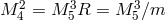
As explained in [293*], in the case where there is a large Hierarchy between the two Planck scales
,
As explained in [293*], in the case where there is a large Hierarchy between the two Planck scales ![(2) ∫ [ 1 [ 1 ( )] Sbi−gravity = d4x− -hμν ℰˆμανβ+ -m2eff δαμ δβν − η αβημν h αβ (5.51 ) 4 ] 2 − 1ℓμν ˆℰαβℓ . 4 μν αβ](article836x.gif)
 and
and
 , the massive particles is always the one that enters at the lower Planck mass and the massless one the
one that has a large Planck scale. For instance if
, the massive particles is always the one that enters at the lower Planck mass and the massless one the
one that has a large Planck scale. For instance if  , the massless particle is mainly given by
 and the massive one mainly by
  . This means that in the limit
  while keeping
  fixed, we recover the theory of a massive gravity and a fully decoupled massless graviton as will be
explained in Section 8.2.
fixed, we recover the theory of a massive gravity and a fully decoupled massless graviton as will be
explained in Section 8.2.
5.5 Coupling to matter
So far we have only focus on an empty five-dimensional bulk with no matter. It is natural, though, to
consider matter fields living in five dimensions,  with Lagrangian (in the gauge choice (5.7*))

 copies
for
copies
for 
 and each field
  is coupled to the associated vielbein
  or metric
 at the same site. In the discretization procedure, the gradient along the extra dimension
yields a mixing (interaction) between fields located on neighboring sites,
(assuming again periodic boundary conditions,
at the same site. In the discretization procedure, the gradient along the extra dimension
yields a mixing (interaction) between fields located on neighboring sites,
(assuming again periodic boundary conditions, 
 ). The discretization procedure could be also
performed using a more complicated definition of the derivative along
). The discretization procedure could be also
performed using a more complicated definition of the derivative along  involving more than two sites,
which leads to further interactions between the different fields.
involving more than two sites,
which leads to further interactions between the different fields.
In the two-sight derivative formulation, the action for matter is then
The coupling to gauge fields or fermions can be derived in the same way, and the vielbein formalism makes it natural to extend the action (5.6*) to five dimensions and applying the discretization procedure. Interestingly, in the case of fermions, the fields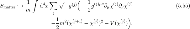
 and
and  would not directly couple to one another,
but they would couple to both the vielbein
would not directly couple to one another,
but they would couple to both the vielbein  at the same site and the one
  on the neighboring
site.
on the neighboring
site.
Notice, however, that the current full proofs for the absence of the BD ghost do not include such couplings between matter fields living on different metrics (or vielbeins), nor matter fields coupling directly to more than one metric (vielbein).
5.6 No new kinetic interactions
In GR, diffeomorphism invariance uniquely fixes the kinetic term to be the Einstein–Hilbert one
(see, for instance, Refs. [287, 483, 175, 225, 76] for the uniqueness of GR for the theory of a massless spin-2 field).
In more than four dimensions, the GR action can be supplemented by additional Lovelock invariants [383] which respect diffeomorphism invariance and are expressed in terms of higher powers of the Riemann curvature but lead to second order equations of motion. In four dimensions there is only one non-trivial additional Lovelock invariant corresponding the Gauss–Bonnet term but it is topological and thus does not affect the theory, unless other degrees of freedom such as a scalar field is included.
So, when dealing with the theory of a single massless spin-2 field in four dimensions the only allowed kinetic term is the well-known Einstein–Hilbert one. Now when it comes to the theory of a massive spin-2 field, diffeomorphism invariance is broken and so in addition to the allowed potential terms described in (6.9*) – (6.13*), one could consider other kinetic terms which break diffeomorphism.
This possibility was explored in Refs. [231*, 310*, 230] where it was shown that in four dimensions, the
following derivative interaction  is ghost-free at leading order (i.e., there is no higher derivatives for
the Stückelberg fields when introducing the Stückelberg fields associated with linear diffeomorphism),
is ghost-free at leading order (i.e., there is no higher derivatives for
the Stückelberg fields when introducing the Stückelberg fields associated with linear diffeomorphism),

Now let us turn to a theory of gravity. In that case, we have seen that the coupling to matter forces
linear diffeomorphisms to be extended to fully non-linear diffeomorphism. So to be viable in a
theory of massive gravity, the derivative interaction (5.57*) should enjoy a ghost-free non-linear
completion (the absence of ghost non-linearly can be checked for instance by restoring non-linear
diffeomorphism using the non-linear Stückelberg decomposition (2.80*) in terms of the helicity-1 and -0
modes given in (2.46*), or by performing an ADM analysis as will be performed for the mass
term in Section 7.) It is easy to check that by itself  has a ghost at quartic order and
so other non-linear interactions should be included for this term to have any chance of being
ghost-free.
has a ghost at quartic order and
so other non-linear interactions should be included for this term to have any chance of being
ghost-free.
Within the deconstruction paradigm, the non-linear completion of  could have a natural
interpretation as arising from the five-dimensional Gauss–Bonnet term after discretization. Exploring the
avenue would indeed lead to a new kinetic interaction of the form
could have a natural
interpretation as arising from the five-dimensional Gauss–Bonnet term after discretization. Exploring the
avenue would indeed lead to a new kinetic interaction of the form  , where
  is the
dual Riemann tensor [339*, 153*]. However, a simple ADM analysis shows that such a term propagates
more than five degrees of freedom and thus has an Ostrogradsky ghost (similarly as the BD
ghost). As a result this new kinetic interaction (5.57*) does not have a natural realization from
a five-dimensional point of view (at least in its metric formulation, see Ref. [153*] for more
details.)
is the
dual Riemann tensor [339*, 153*]. However, a simple ADM analysis shows that such a term propagates
more than five degrees of freedom and thus has an Ostrogradsky ghost (similarly as the BD
ghost). As a result this new kinetic interaction (5.57*) does not have a natural realization from
a five-dimensional point of view (at least in its metric formulation, see Ref. [153*] for more
details.)
We can push the analysis even further and show that no matter what the higher order interactions are,
as soon as  is present it will always lead to a ghost and so such an interaction is never
acceptable [153*].
is present it will always lead to a ghost and so such an interaction is never
acceptable [153*].
As a result, the Einstein–Hilbert kinetic term is the only allowed kinetic term in Lorentz-invariant (massive) gravity.
This result shows how special and unique the Einstein–Hilbert term is. Even without imposing diffeomorphism invariance, the stability of the theory fixes the kinetic term to be nothing else than the Einstein–Hilbert term and thus forces diffeomorphism invariance at the level of the kinetic term. Even without requiring coordinate transformation invariance, the Riemann curvature remains the building block of the kinetic structure of the theory, just as in GR.
Before summarizing the derivation of massive gravity from higher dimensional deconstruction / Kaluza–Klein
decomposition, we briefly comment on other ‘apparent’ modifications of the kinetic structure like in  – gravity (see for instance Refs. [89*, 354*, 46*] for
  massive gravity and their implications to
cosmology).
massive gravity and their implications to
cosmology).
Such kinetic terms à la  are also possible without a mass term for the graviton. In that case
diffeomorphism invariance allows us to perform a change of frame. In the Einstein-frame
are also possible without a mass term for the graviton. In that case
diffeomorphism invariance allows us to perform a change of frame. In the Einstein-frame  gravity is
seen to correspond to a theory of gravity with a scalar field, and the same result will hold in
gravity is
seen to correspond to a theory of gravity with a scalar field, and the same result will hold in  massive
gravity (in that case the scalar field couples non-trivially to the Stückelberg fields). As a result
massive
gravity (in that case the scalar field couples non-trivially to the Stückelberg fields). As a result  is
not a genuine modification of the kinetic term but rather a standard Einstein–Hilbert term and the addition
of a new scalar degree of freedom which not a degree of freedom of the graviton but rather an independent
scalar degree of freedom which couples non-minimally to matter (see Ref. [128] for a review on
is
not a genuine modification of the kinetic term but rather a standard Einstein–Hilbert term and the addition
of a new scalar degree of freedom which not a degree of freedom of the graviton but rather an independent
scalar degree of freedom which couples non-minimally to matter (see Ref. [128] for a review on
 -gravity.)
 |
 |
 |
Living Rev. Relativity, 17 (2014), 7, doi:10.12942/lrr-2014-7, URL (accessed <date>): http://www.livingreviews.org/lrr-2014-7.
 This work is licensed under a Creative Commons License.
© The author(s), except where otherwise noted.
This work is licensed under a Creative Commons License.
© The author(s), except where otherwise noted.