 -decoupling
limit of bi-gravity
-decoupling
limit of bi-gravity
 )
)12 Cosmology
One of the principal motivations for considering massive theories of gravity is their potential to address, or at least provide a new perspective on, the issue of cosmic acceleration as already discussed in Section 3. Adding a mass for the graviton keeps physics at small scales largely equivalent to GR because of the Vainshtein mechanism. However, it inevitably modifies gravity in at large distances, i.e., in the infrared. This modification of gravity is thus most significant for sources which are long wavelength. The cosmological constant is the most infrared source possible since it is build entirely out of zero momentum modes and for this reason we may hope that the nature of a cosmological constant in a theory of massive gravity or similar infrared modification is changed.There have been two principal ideas for how massive theories of gravity could be useful for addressing the cosmological constant. On the one hand, by weakening gravity in the infrared, they may weaken the sensitivity of the dynamics to an already existing large cosmological constant. This is the idea behind screening or degravitating solutions [211, 212, 26, 216] (see Section 4.5). The second idea is that a condensate of massive gravitons could form which act as a source for self-acceleration, potentially explaining the current cosmic acceleration without the need to introduce a non-zero cosmological constant (as in the case of the DGP model [159, 163], see Section 4.4). This idea does not address the ‘old cosmological constant problem’ [484*] but rather assumes that some other symmetry, or mechanism exists which ensures the vacuum energy vanishes. Given this, massive theories of gravity could potential provide an explanation for the currently small, and hence technically unnatural value of the cosmological constant, by tying it to the small, technically natural, value of the graviton mass.
Thus, the idea of screening/degravitation and self-acceleration are logically opposites to each other, but there is some evidence that both can be achieved in massive theories of gravity. This evidence is provided by the decoupling limit of massive gravity to which we review first. We then go on to discuss attempts to find exact solutions in massive gravity and its various extensions.
12.1 Cosmology in the decoupling limit
A great deal of understanding about the cosmological solutions in massive gravity theories can be
learned from considering the ‘decoupling limit’ of massive gravity discussed in Section 8.3. The
idea here is to recognize that locally, i.e., in the vicinity of a point, any FLRW geometry can
be expressed as a small perturbation about Minkowski spacetime (about  ) with the
perturbation expansion being good for distances small relative to the curvature radius of the geometry:
) with the
perturbation expansion being good for distances small relative to the curvature radius of the geometry:
![[ ] [ 1 ] ds2 = − 1 − (H˙ + H2 )⃗x2 dt2 + 1 − -H2 ⃗x2 d⃗x2 (12.1 ) ( ) 2 1 FLRW μ ν = ημν + M---hμν dx dx . (12.2 ) Pl](article2292x.gif)
 ,
,  we keep the canonically normalized metric perturbation
 fixed. Thus, the decoupling limit corresponds to keeping
  and
and  fixed, or equivalently
 and
and  fixed. Despite the fact that
  vanishes in this limit, the analogue of the
Friedmann equation remains nontrivial if we also scale the energy density such that
vanishes in this limit, the analogue of the
Friedmann equation remains nontrivial if we also scale the energy density such that  remains finite.
Because of this fact, it is possible to analyze the modification to the Friedmann equation in the decoupling
limit.31
remains finite.
Because of this fact, it is possible to analyze the modification to the Friedmann equation in the decoupling
limit.31
The generic form for the helicity-0 mode which preserves isotropy near  is
is

 , this also preserves homogeneity in a theory in which the Galileon
symmetry is exact, as in massive gravity, since a translation in
, this also preserves homogeneity in a theory in which the Galileon
symmetry is exact, as in massive gravity, since a translation in  corresponds to a Galileon transformation
of
corresponds to a Galileon transformation
of  which leaves invariant the combination
  . In Ref. [139*] this ansatz was used to derive the
existence of both self-accelerating and screening solutions.
. In Ref. [139*] this ansatz was used to derive the
existence of both self-accelerating and screening solutions.
Friedmann equation in the decoupling limit
We start with the decoupling limit Lagrangian given in (8.38*). Following the same notation as in Ref. [139]
we set  , where the coefficients
  are given in terms of the
  ’s in (8.47*). The
self-accelerating branch of solutions then corresponds to the ansatz
’s in (8.47*). The
self-accelerating branch of solutions then corresponds to the ansatz
 and
and  correspond to the fluctuations about the background solution.
For this ansatz, the background equations of motion reduce to
In the ‘self-accelerating branch’ when
 , the first constraint can be used to infer
  and the
second one corresponds to the effective Friedmann equation. We see that even in the absence of a
cosmological constant
and the
second one corresponds to the effective Friedmann equation. We see that even in the absence of a
cosmological constant  , for generic coefficients we have a constant
  solution which corresponds
to a self-accelerating de Sitter solution.
solution which corresponds
to a self-accelerating de Sitter solution.
The stability of these solutions can be analyzed by looking at the Lagrangian for the quadratic fluctuations
Thus, we see that the helicity zero mode is stable provided that However, these solutions exhibit a peculiarity. To this order, the helicity-0 mode fluctuations do not couple to the matter perturbations (there is no kinetic mixing between

 and
and  ). This means that there is
no Vainshtein effect, but at the same time there is no vDVZ discontinuity for the Vainshtein effect to
resolve!
). This means that there is
no Vainshtein effect, but at the same time there is no vDVZ discontinuity for the Vainshtein effect to
resolve!
Screening solution
Another way to solve the system of Eqs. (12.7*) and (12.8*) is to consider instead flat solutions
 . Then (12.7*) is trivially satisfied and we see the existence of a ‘screening solution’
in the Friedmann equation (12.8*), which can accommodate a cosmological constant without
any acceleration. This occurs when the helicity-0 mode ‘absorbs’ the contribution from the
cosmological constant
. Then (12.7*) is trivially satisfied and we see the existence of a ‘screening solution’
in the Friedmann equation (12.8*), which can accommodate a cosmological constant without
any acceleration. This occurs when the helicity-0 mode ‘absorbs’ the contribution from the
cosmological constant  , and the background configuration for
  parametrized by
  satisfies


 , they correspond to Minkowski solutions which are sourced by a nonzero cosmological
constant. In the case where
, they correspond to Minkowski solutions which are sourced by a nonzero cosmological
constant. In the case where  , these solutions only exist if
  . In the case where
 , there is no upper bound on the cosmological constant which can be screened via this
mechanism.
, there is no upper bound on the cosmological constant which can be screened via this
mechanism.
In this branch of solution, the strong coupling scale for fluctuations on top of this configuration becomes of the same order of magnitude as that of the screened cosmological constant. For a large cosmological constant the strong coupling scale becomes to large and the helicity-0 mode would thus not be sufficiently Vainshtein screened.
Thus, while these solutions seem to indicate positively that there are self-screening solutions which can accommodate a continuous range of values for the cosmological constant and still remain flat, the range is too small to significantly change the old cosmological constant problem. Nevertheless, the considerable difficulty in attacking the old cosmological constant problem means that these solutions deserve further attention as they also provide a proof of principle on how Weinberg’s no go could be evaded [484]. We emphasize that what prevents a large cosmological constant from being screened is not an issue in the theoretical tuning but rather an observational bound, so this is already a step forward.
These two classes of solutions are both maximally symmetric. However, the general cosmological
solution is isotropic but inhomogeneous. This is due to the fact that a nontrivial time dependence
for the matter source will inevitably source  , and as soon as
  the solutions are
inhomogeneous. In fact, as we now explain in general, the full nonlinear solution is inevitably
inhomogeneous due to the existence of a no-go theorem against spatially flat and closed FLRW
solutions.
the solutions are
inhomogeneous. In fact, as we now explain in general, the full nonlinear solution is inevitably
inhomogeneous due to the existence of a no-go theorem against spatially flat and closed FLRW
solutions.
12.2 FLRW solutions in the full theory
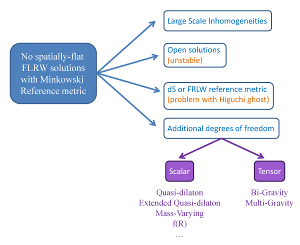
12.2.1 Absence of flat/closed FLRW solutions
A nontrivial consequence of the fact that diffeomorphism invariance is broken in massive gravity is
that there are no spatially flat or closed FLRW solutions [117*]. This result follows from the
different nature of the Hamiltonian constraint. For instance, choosing a spatially flat form for the
metric  , the mini-superspace Lagrangian takes the schematic form

 and the acceleration
equation for
and the acceleration
equation for  implies
In GR, since
implies
In GR, since 
 , there is no analogue of this equation. In the present case, this equation can be
solved either by imposing
, there is no analogue of this equation. In the present case, this equation can be
solved either by imposing  which implies the absence of any dynamic FLRW solutions, or by solving
 for fixed
  which implies the same thing. Thus, there are no nontrivial spatially flat FLRW
solutions in massive gravity in which the reference metric is Minkowski. The result extends also to
spatially closed cosmological solutions. As a result, different alternatives have been explored in the
literature to study the cosmology of massive gravity. See Figure 7* for a summary of these different
approaches.
which implies the same thing. Thus, there are no nontrivial spatially flat FLRW
solutions in massive gravity in which the reference metric is Minkowski. The result extends also to
spatially closed cosmological solutions. As a result, different alternatives have been explored in the
literature to study the cosmology of massive gravity. See Figure 7* for a summary of these different
approaches.
12.2.2 Open FLRW solutions
While the previous argument rules out the possibility of spatially flat and closed FLRW solutions, open ones
are allowed [283]. To see this we make the ansatz  , where
  expressed in
the form
expressed in
the form

 with
then the mini-superspace Lagrangian of (6.3*) takes the form
with
with
then the mini-superspace Lagrangian of (6.3*) takes the form
with 
![aa˙2 [ ∘ --- ℒmGR = − 3M 2Pl|k|N a − 3M P2l----+ 3m2M 2Pl2a2 𝒳(2N a − f˙a − N |k|f N ∘ --- ] + α3a2𝒳 2(4N a − 3f˙a − N |k |f ) + 4α4a3 𝒳 3(N − f˙) ,](article2350x.gif)
 . In this case, the analogue additional constraint imposed by consistency of the
Friedmann and acceleration (Raychaudhuri) equation is
The solution for which
. In this case, the analogue additional constraint imposed by consistency of the
Friedmann and acceleration (Raychaudhuri) equation is
The solution for which 
 is essentially Minkowski spacetime in the open slicing, and is thus
uninteresting as a cosmology.
is essentially Minkowski spacetime in the open slicing, and is thus
uninteresting as a cosmology.
Focusing on the other branch and assuming  , the general solution determines
  in terms of
 takes the form
  where
where  is a constant determined by the quadratic equation


12.3 Inhomogenous/anisotropic cosmological solutions
As pointed out in [117], the absence of FLRW solutions in massive gravity should not be viewed as
an observational flaw of the theory. On the contrary, the Vainshtein mechanism guarantees
that there exist inhomogeneous cosmological solutions which approximate the normal FLRW
solutions of GR as closely as desired in the limit  . Rather, it is the existence of a new
physical length scale
. Rather, it is the existence of a new
physical length scale  in massive gravity, which cause the dynamics to be inhomogeneous at
cosmological scales. If this scale
in massive gravity, which cause the dynamics to be inhomogeneous at
cosmological scales. If this scale  is comparable to or larger than the current Hubble
radius, then the effects of these inhomogeneities would only become apparent today, with the
universe locally appearing as homogeneous for most of its history in the local patch that we
observe.
is comparable to or larger than the current Hubble
radius, then the effects of these inhomogeneities would only become apparent today, with the
universe locally appearing as homogeneous for most of its history in the local patch that we
observe.
One way to understand how the Vainshtein mechanism recovers the prediction of homogeneity and
isotropy is to work in the formulation of massive gravity in which the Stückelberg fields are turned on. In
this formulation, the Stückelberg fields can exhibit order unity inhomogeneities with the metric remaining
approximately homogeneous. Matter that couples only to the metric will perceive an effectively
homogeneous and anisotropic universe, and only through interaction with the Vainshtein suppressed
additional scalar and vector degrees of freedom would it be possible to perceive the inhomogeneities. This is
achieved because the metric is sourced by the Stückelberg fields through terms in the equations of
motion which are suppressed by  . Thus, as long as
  , the metric remains effectively
homogeneous and isotropic despite the existence of no-go theorems against exact homogeneity and
isotropy.
, the metric remains effectively
homogeneous and isotropic despite the existence of no-go theorems against exact homogeneity and
isotropy.
In this regard, a whole range of exact solutions have been studied exhibiting these properties [364, 474*, 363, 97, 264, 356, 456, 491, 476*, 334, 478*, 265, 124, 123*, 125, 455, 198]. A generalization of some of these solutions was presented in Ref. [404] and Ref. [266]. In particular, we note that in [475*, 476] the most general exact solution of massive gravity is obtained in which the metric is homogeneous and isotropic with the Stückelberg fields inhomogeneous. These solutions exist because the effective contribution to the stress energy tensor from the mass term (i.e., viewing the mass term corrections as a modification to the energy density) remains homogeneous and isotropic despite the fact that it is build out of Stückelberg fields which are themselves inhomogeneous.
Let us briefly discuss how these solutions are
obtained.32
As we have already discussed, all solutions of massive gravity can be seen as  decoupling limits
of bi-gravity. Therefore, we may consider the case of inhomogeneous solutions in bi-gravity and the solutions
of massive gravity can always be derived as a limit of these bi-gravity solutions. We thus begin with the
action
decoupling limits
of bi-gravity. Therefore, we may consider the case of inhomogeneous solutions in bi-gravity and the solutions
of massive gravity can always be derived as a limit of these bi-gravity solutions. We thus begin with the
action
![2 ∫ 2 ∫ ∘ ---- S = M-Pl d4x√ −-gR [g] + M-f- d4x − f R[f] (12.22 ) 2 2 m2M 2 ∫ √ ---∑ βn √ -- + -----eff d4x − g --ℒn ( 𝕏 ) + Matter, 4 n n!](article2371x.gif)
 and
and  and we may imagine matter coupled to both
  and
and  but for simplicity let us imagine matter is either minimally coupled to
  or it is minimally coupled to
 .
.
12.3.1 Special isotropic and inhomogeneous solutions
Although it is possible to find solutions in which the two metrics are proportional to each other
 [478*], these solutions require in addition that the stress energies of matter sourcing
 and
and  are proportional to one another. This is clearly too restrictive a condition to be
phenomenologically interesting. A more general and physically realistic assumption is to suppose
that both metrics are isotropic but not necessarily homogeneous. This is covered by the ansatz
are proportional to one another. This is clearly too restrictive a condition to be
phenomenologically interesting. A more general and physically realistic assumption is to suppose
that both metrics are isotropic but not necessarily homogeneous. This is covered by the ansatz
 is the metric on a unit 2-sphere. To put the
  metric in diagonal form we have made use of
the one copy of overall diff invariance present in bi-gravity. To distinguish from the bi-diagonal case we shall
assume that
metric in diagonal form we have made use of
the one copy of overall diff invariance present in bi-gravity. To distinguish from the bi-diagonal case we shall
assume that  . The bi-diagonal case allows for homogeneous and isotropic solutions for both
metrics which will be dealt with in Section 12.4.2. The square root may be easily taken to give
which can easily be used to determine the contribution of the mass terms to the equations of motion for
. The bi-diagonal case allows for homogeneous and isotropic solutions for both
metrics which will be dealt with in Section 12.4.2. The square root may be easily taken to give
which can easily be used to determine the contribution of the mass terms to the equations of motion for
 and
and  . This leads to a set of partial differential equations for
  which in
general require numerical analysis. As in GR, due to the presence of constraints associated with
diffeomorphism invariance, and the Hamiltonian constraint for the massive graviton, several of
these equations will be first order in time-derivatives. This simplifies matters somewhat but not
sufficiently to make analytic progress. Analytic progress can be made however by making additional
more restrictive assumptions, at the cost of potentially losing the most physically interesting
solutions.
which in
general require numerical analysis. As in GR, due to the presence of constraints associated with
diffeomorphism invariance, and the Hamiltonian constraint for the massive graviton, several of
these equations will be first order in time-derivatives. This simplifies matters somewhat but not
sufficiently to make analytic progress. Analytic progress can be made however by making additional
more restrictive assumptions, at the cost of potentially losing the most physically interesting
solutions.
Effective cosmological constant
For instance, from the above form we may determine that the effective contribution to the stress energy
tensor sourcing  arising from the mass term is of the form

 is of the FLRW form or is static, then
this requires that
is of the FLRW form or is static, then
this requires that  =0 which for
  implies
This should be viewed as an equation for
implies
This should be viewed as an equation for 
 whose solution is
Then conservation of energy imposes further
since
whose solution is
Then conservation of energy imposes further
since 
 is already fixed we should view this generically as an equation for
  in terms of
  and
and  With these assumptions the contribution of the mass term to the effective stress energy tensor sourcing each
metric becomes equivalent to a cosmological constant for each metric
With these assumptions the contribution of the mass term to the effective stress energy tensor sourcing each
metric becomes equivalent to a cosmological constant for each metric 
 and
and
 with
Thus, all of the potential dynamics of the mass term is reduced to an effective cosmological constant. Let us
stress again that this rather special fact is dependent on the rather restrictive assumptions imposed on the
metric
with
Thus, all of the potential dynamics of the mass term is reduced to an effective cosmological constant. Let us
stress again that this rather special fact is dependent on the rather restrictive assumptions imposed on the
metric 
 and that we certainly do not expect this to be the case for the most general time-dependent,
isotropic, inhomogeneous solution.
and that we certainly do not expect this to be the case for the most general time-dependent,
isotropic, inhomogeneous solution.
Massive gravity limit
As usual, we can take the  limit to recover solutions for massive gravity on Minkowski (if
 ) or more generally if the scaling of the parameters
  is chosen so that
  and
and
 and hence
  remains finite in the limit then these will give rise to
solutions for massive gravity for which the reference metric is any Einstein space for which
remains finite in the limit then these will give rise to
solutions for massive gravity for which the reference metric is any Einstein space for which

Thus, for example, assuming no additional matter couples to the  metric, both bi-gravity and
massive gravity on a fixed reference metric admit exact cosmological solutions for which the
metric, both bi-gravity and
massive gravity on a fixed reference metric admit exact cosmological solutions for which the  metric is
de Sitter or anti-de Sitter
metric is
de Sitter or anti-de Sitter
 , and the scale factor
  satisfies
where
satisfies
where 
 is the energy density of matter minimally coupled to
  ,
,  , and
, and  can be
expressed as a function of
can be
expressed as a function of  and
and  and comparing with the previous representation
  . The one
remaining undetermined function is
. The one
remaining undetermined function is  and this is determined by the constraint that
 and the conversion relations
which determine
and the conversion relations
which determine 
 and
and  in terms of
  and
and  . These relations are difficult to solve
exactly, but if we consider the special case
. These relations are difficult to solve
exactly, but if we consider the special case  which corresponds in particular to massive gravity on
Minkowski then the solution is
where
which corresponds in particular to massive gravity on
Minkowski then the solution is
where 
 is an integration constant.
In particular, in the open universe case  ,
,  ,
,  ,
,  , we recover the
open universe solution of massive gravity considered in Section 12.2.2, where for comparison
, we recover the
open universe solution of massive gravity considered in Section 12.2.2, where for comparison
 ,
,  and
and  .
.
12.3.2 General anisotropic and inhomogeneous solutions
Let us reiterate again that there are a large class of inhomogeneous but isotropic cosmological solutions for
which the effective Friedmann equation for the  metric is the same as in GR with just the addition of a
cosmological constant which depends on the graviton mass parameters. However, these are not the most
general solutions, and as we have already discussed many of the exact solutions of this form considered so
far have been found to be unstable, in particular through the absence of kinetic terms for degrees of freedom
which implies infinite strong coupling. However, all the exact solutions arise from making a strong
restriction on one or the other of the metrics which is not expected to be the case in general. Thus,
the search for the ‘correct’ cosmological solution of massive gravity and bi-gravity will almost
certainly require a numerical solution of the general equations for
metric is the same as in GR with just the addition of a
cosmological constant which depends on the graviton mass parameters. However, these are not the most
general solutions, and as we have already discussed many of the exact solutions of this form considered so
far have been found to be unstable, in particular through the absence of kinetic terms for degrees of freedom
which implies infinite strong coupling. However, all the exact solutions arise from making a strong
restriction on one or the other of the metrics which is not expected to be the case in general. Thus,
the search for the ‘correct’ cosmological solution of massive gravity and bi-gravity will almost
certainly require a numerical solution of the general equations for  , and their
stability.
, and their
stability.
Closely related to this, we may consider solutions which maintain homogeneity, but are anisotropic [284*, 393*, 123*]. In [393] the general Bianchi class A cosmological solutions in bi-gravity are studied. There it is shown that the generic anisotropic cosmological solution in bi-gravity asymptotes to a self-accelerating solution, with an acceleration determined by the mass terms, but with an anisotropy that falls off less rapidly than in GR. In particular the anisotropic contribution to the effective energy density redshifts like non-relativistic matter. In [284, 123] it is found that if the reference metric is made to be of an anisotropic FLRW form, then for a range of parameters and initial conditions stable ghost free cosmological solutions can be found.
These analyses are ongoing and it has been uncovered that certain classes of exact solutions exhibit strong coupling instabilities due to vanishing kinetic terms and related pathologies. However, this simply indicates that these solutions are not good semi-classical backgrounds. The general inhomogeneous cosmological solution (for which the metric is also inhomogeneous) is not known at present, and it is unlikely it will be possible to obtain it exactly. Thus, it is at present unclear what are the precise nonlinear completions of the stable inhomogeneous cosmological solutions that can be found in the decoupling limit. Thus the understanding of the cosmology of massive gravity should be regarded as very much work in progress, at present it is unclear what semi-classical solutions of massive gravity are the most relevant for connecting with our observed cosmological evolution.
12.4 Massive gravity on FLRW and bi-gravity
12.4.1 FLRW reference metric
One straightforward extension of the massive gravity framework is to allow for modifications to the reference metric, either by making it cosmological or by extending to bi-gravity (or multi-gravity). In the former case, the no-go theorem is immediately avoided since if the reference metric is itself an FLRW geometry, there can no longer be any obstruction to finding FLRW geometries.
The case of massive gravity with a spatially flat FLRW reference metric was worked out in [223*], where
it was found that if using the convention for which the massive gravity Lagrangian is (6.5*) with the
potential given in terms of the coefficient  as in (6.23*), then the Friedmann equation takes the form


 is the Hubble parameter for the reference metric. By itself, this Friedmann equation looks
healthy in the sense that it admits FLRW solutions that can be made as close as desired to the usual
solutions of GR.
is the Hubble parameter for the reference metric. By itself, this Friedmann equation looks
healthy in the sense that it admits FLRW solutions that can be made as close as desired to the usual
solutions of GR.
However, in practice, the generalization of the Higuchi consideration [307] to this case leads to an unacceptable bound (see Section 8.3.6).
It is a straightforward consequence of the representation theory for the de Sitter group that a unitary
massive spin-2 representation only exists in four dimensions for  as was the case in de Sitter.
Although this result only holds for linearized fluctuations around de Sitter, its origin as a bound comes
from the requirement that the kinetic term for the helicity zero mode is positive, i.e., the absence of ghosts
in the scalar perturbations sector. In particular, the kinetic term for the helicity-0 mode
as was the case in de Sitter.
Although this result only holds for linearized fluctuations around de Sitter, its origin as a bound comes
from the requirement that the kinetic term for the helicity zero mode is positive, i.e., the absence of ghosts
in the scalar perturbations sector. In particular, the kinetic term for the helicity-0 mode  takes the form

This generalized bound was worked out in [223] and takes the form
Again, by itself this equation is easy to satisfy. However, combined with the Friedmann equation, we see that the two equations are generically in conflict if in addition we require that the massive gravity corrections to the Friedmann equation are small for most of the history of the Universe, i.e., during radiation and matter domination This phenomenological requirement essentially rules out the applicability of FLRW cosmological solutions in massive gravity with an FLRW reference metric.![2 [ 2] − -m----H- 3β + 4β H--+ β H-- ≥ 2H2. (12.48 ) 4M 2PlHf 1 2Hf 3H2f](article2456x.gif)

This latter problem which is severe for massive gravity with dS or FLRW reference metrics,33 gets resolved in bi-gravity extensions, at least for a finite regime of parameters.
12.4.2 Bi-gravity
Cosmological solutions in bi-gravity have been considered in [474, 479, 104, 106*, 8*, 475, 478, 9*, 7, 62*].
We keep the same notation as previously and consider the action for bi-gravity as in (5.43*) (in
terms of the  ’s where the conversion between the
  ’s and the
  ’s is given in (6.28*))
![2 √ --- M 2∘ ---- ℒbi−gravity = M-Pl − gR [g] +--f- − f R[f] 2 2 m2M 2 ∑4 βn √ -- + -----Pl ---ℒn[ 𝕏 ] + ℒmatter[g,ψi], (12.50 ) 4 n=0 n!](article2461x.gif)
 metric. Then the two Friedmann equations for each Hubble
parameter take the respective form
Crucially, the generalization of the Higuchi bound now becomes
The important new feature is the last term in square brackets. Although this tends to unity in
the limit
metric. Then the two Friedmann equations for each Hubble
parameter take the respective form
Crucially, the generalization of the Higuchi bound now becomes
The important new feature is the last term in square brackets. Although this tends to unity in
the limit ![( ) 2 ∑3 3(4 − n)m2 βn H n 1 H = − -------------- --- + ---2-ρ (12.51 ) n=0 [ 2n! Hf 3]M Pl 2 ∑3 2 ( )n− 3 H2f = − M-Pl 3m--βn+1- H-- . (12.52 ) M f2 n=0 2n! Hf](article2463x.gif)
![[ ] [ ] m2 H H H2 ( Hf MPl )2 − ------ 3β1 + 4β2--- + β3 --2 1 + ------- ≥ 2H2. (12.53 ) 4 Hf Hf H f HMf](article2464x.gif)
 , which is consistent with the massive gravity result, for finite
  it
opens a new regime where the bound is satisfied by having
it
opens a new regime where the bound is satisfied by having  (notice that in our
convention the
(notice that in our
convention the  ’s are typically negative). One may show [224] that it is straightforward to
find solutions of both Friedmann equations which are consistent with the Higuchi bound over
the entire history of the universe. For example, choosing the parameters
’s are typically negative). One may show [224] that it is straightforward to
find solutions of both Friedmann equations which are consistent with the Higuchi bound over
the entire history of the universe. For example, choosing the parameters  and
solving for
and
solving for  the effective Friedmann equation for the metric which matter couples to is
and the generalization of the Higuchi bound is
which is trivially satisfied at all times. More generally, there is an open set of such solutions. The
observationally viability of the self-accelerating branch of these models has been considered in [8, 9] with
generally positive results. Growth histories of the bi-gravity cosmological solutions have been
considered in [62]. However, while avoiding the Higuchi bound indicates absence of ghosts, it
has been argued that these solutions may admit gradient instabilities in their cosmological
perturbations [106].
the effective Friedmann equation for the metric which matter couples to is
and the generalization of the Higuchi bound is
which is trivially satisfied at all times. More generally, there is an open set of such solutions. The
observationally viability of the self-accelerating branch of these models has been considered in [8, 9] with
generally positive results. Growth histories of the bi-gravity cosmological solutions have been
considered in [62]. However, while avoiding the Higuchi bound indicates absence of ghosts, it
has been argued that these solutions may admit gradient instabilities in their cosmological
perturbations [106].


We should stress again that just as in massive gravity, the absence of FLRW solutions should not be viewed as an inconsistency of the theory with observations, also in bi-gravity these solutions may not necessarily be the ones of most relevance for connecting with observations. It is only that they are the most straightforward to obtain analytically. Thus, cosmological solutions in bi-gravity, just as in massive gravity, should very much be viewed as a work in progress.
12.5 Other proposals for cosmological solutions
Finally, we may note that more serious modifications the massive gravity framework have been considered in order to allow for FLRW solutions. These include mass-varying gravity and the quasi-dilaton models [119*, 118]. In [281] it was shown that mass-varying gravity and the quasi-dilaton model could allow for stable cosmological solutions but for the original quasi-dilaton theory the self-accelerating solutions are always unstable. On the other hand, the generalizations of the quasi-dilaton [126*, 127*] appears to allow stable cosmological solutions.
In addition, one can find cosmological solutions in non-Lorentz invariant versions of massive
gravity [109*] (and [103, 107*, 108*]). We can also allow the mass to become dependent on a field [489, 375],
extend to multiple metrics/vierbeins [454], extensions with  terms either in massive gravity [89] or
in bi-gravity [416, 415] which leads to interesting self-accelerating solutions. Alternatively, one can
consider other extensions to the form of the mass terms by coupling massive gravity to the DBI
Galileons [237, 19, 20, 315].
terms either in massive gravity [89] or
in bi-gravity [416, 415] which leads to interesting self-accelerating solutions. Alternatively, one can
consider other extensions to the form of the mass terms by coupling massive gravity to the DBI
Galileons [237, 19, 20, 315].
As an example, we present here the cosmology of the extension of the quasi-dilaton model considered
in [127*], where the reference metric  is given in (9.15*) and depends explicitly on the dynamical
quasi-dilaton field
is given in (9.15*) and depends explicitly on the dynamical
quasi-dilaton field  .
.
The action takes the familiar form with an additional kinetic term introduced for the quasi-dilaton which respects the global symmetry
where the tensor![∫ √ ---[ 1 ω S = M 2Pl d4x − g -R − Λ − ----2(∂ σ)2 2 2M Pl ] m2 ( ) + --- ℒ2[&tidle;𝒦] + α3ℒ3 [𝒦&tidle;] + α4 ℒ4[&tidle;𝒦 ] , (12.56 ) 4](article2476x.gif)
 is given in (9.14*).
The background ansatz is taken as
so that The equation that for normal massive gravity forbids FLRW solutions follows from varying with respect to
 and takes the form
where
As the universe expands
and takes the form
where
As the universe expands 

 which for one branch of solutions implies
  which
determines a fixed constant asymptotic value of
which
determines a fixed constant asymptotic value of  from
from  . In this asymptotic limit the effective
Friedmann equation becomes
where
defines an effective cosmological constant which gives rise to self-acceleration even when
. In this asymptotic limit the effective
Friedmann equation becomes
where
defines an effective cosmological constant which gives rise to self-acceleration even when 
![[ ] ΛX = m2 (X − 1) 6 − 3X + 3(X − 4)(X − 1)α3 + 6(X − 1)2α4 , (12.66 ) 2](article2488x.gif)
 (for
(for
 ).
).
The analysis of [127] shows that these self-accelerating cosmological solutions are ghost free provided that
where In particular, this implies that

 which demonstrates that the original quasi-dilaton
model [119, 116] has a scalar (Higuchi type) ghost. The analysis of [126] confirms these properties in a
more general extension of this model.
which demonstrates that the original quasi-dilaton
model [119, 116] has a scalar (Higuchi type) ghost. The analysis of [126] confirms these properties in a
more general extension of this model.
 |
 |
 |
Living Rev. Relativity, 17 (2014), 7, doi:10.12942/lrr-2014-7, URL (accessed <date>): http://www.livingreviews.org/lrr-2014-7.
 This work is licensed under a Creative Commons License.
© The author(s), except where otherwise noted.
This work is licensed under a Creative Commons License.
© The author(s), except where otherwise noted.