Higher-Dimensional Scenarios

3 Higher-Dimensional Scenarios

As seen in Section 2.5, the ‘most natural’ non-linear extension of the Fierz–Pauli mass term bears a ghost. Constructing consistent theories of massive gravity has actually been a challenging task for years, and higher-dimensional scenario can provide excellent frameworks for explicit realizations of massive gravity. The main motivation behind relying on higher dimensional gravity is twofold:

The five-dimensional theory is explicitly covariant.
A massless spin-2 field in five dimensions has five degrees of freedom which corresponds to the correct number of dofs for a massive spin-2 field in four dimensions without the pathological BD ghost.

While string theory and other higher dimensional theories give rise naturally to massive gravitons, they usually include a massless zero-mode. Furthermore, in the simplest models, as soon as the first massive mode is relevant so is an infinite tower of massive (Kaluza–Klein) modes and one is never in a regime where a single massive graviton dominates, or at least this was the situation until the Dvali–Gabadadze–Porrati model (DGP) [208 *, 209 *, 207 *], provided the first explicit model of (soft) massive gravity, based on a higher-dimensional braneworld model.

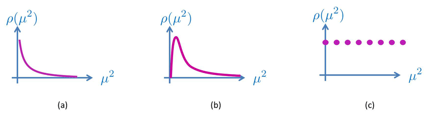
In the DGP model the graviton has a soft mass in the sense that its propagator does not have a simple pole at fixed value $m$ , but rather admits a resonance. Considering the Källén–Lehmann spectral representation [331 , 374 ], the spectral density function $ρ(μ2)$ in DGP is of the form

and so DGP corresponds to a theory of massive gravity with a resonance with width $Δm ∼ m0$ about $m = 0$ .

In a Kaluza–Klein decomposition of a flat extra dimension we have, on the other hand, an infinite tower of massive modes with spectral density function

We shall see in the section on deconstruction (5) how one can truncate this infinite tower by performing a discretization in real space rather than in momentum space à la Kaluza–Klein, so as to obtain a theory of a single massive graviton

or a theory of multi-gravity (with $N$ -interacting gravitons),

In this language, bi-gravity is the special case of multi-gravity where $N = 2$ . These different spectral representations, together with the cascading gravity extension of DGP are represented in Figure 1 *.

Figure 1: Spectral representation of different models. (a) DGP (b) higher-dimensional cascading gravity and (c) multi-gravity. Bi-gravity is the special case of multi-gravity with one massless mode and one massive mode. Massive gravity is the special case where only one massive mode couples to the rest of the standard model and the other modes decouple. (a) and (b) are models of soft massive gravity where the graviton mass can be thought of as a resonance.

Recently, another higher dimensional embedding of bi-gravity was proposed in Ref. [495 ]. Rather than performing a discretization of the extra dimension, the idea behind this model is to consider a two-brane DGP model, where the radion or separation between these branes is stabilized via a Goldberger-Wise stabilization mechanism [255 ] where the brane and the bulk include a specific potential for the radion. At low energy the mass spectrum can be truncated to a massless mode and a massive mode, reproducing a bi-gravity theory. However, the stabilization mechanism involves a relatively low scale and the correspondence breaks down above it. Nevertheless, this provides a first proof of principle for how to embed such a model in a higher-dimensional picture without discretization and could be useful to tackle some of the open questions of massive gravity.

In what follows we review how five-dimensional gravity is a useful starting point in order to generate consistent four-dimensional theories of massive gravity, either for soft-massive gravity à la DGP and its extensions, or for hard massive gravity following a deconstruction framework.

The DGP model has played the role of a precursor for many developments in modified and massive gravity and it is beyond the scope of this review to summarize all of them. In this review we briefly summarize the DGP model and some key aspects of its phenomenology, and refer the reader to other reviews (see for instance [232 , 390 , 234 ]) for more details on the subject.

In this section, $A, B, C ⋅⋅⋅ = 0,...,4$ represent five-dimensional spacetime indices and $μ, ν,α ⋅⋅⋅ = 0,...,3$ label four-dimensional spacetime indices. $y = x4$ represents the fifth additional dimension, $A μ {x } = {x ,y}$ . The five-dimensional metric is given by $(5) gAB (x,y)$ while the four-dimensional metric is given by $gμν(x )$ . The five-dimensional scalar curvature is $(5) R [G ]$ while $R = R [g]$ is the four-dimensional scalar-curvature. We use the same notation for the Einstein tensor where $(5)GAB$ is the five-dimensional one and $Gμν$ represents the four-dimensional one built out of $g μν$ .

When working in the Einstein–Cartan formalism of gravity, $a, b,c,⋅⋅⋅$ label five-dimensional Lorentz indices and $a,b,c⋅⋅⋅$ label the four-dimensional ones.

	Abstract
1	Introduction
2	Massive and Interacting Fields
	2.1	Proca field
	2.2	Spin-2 field
	2.3	From linearized diffeomorphism to full diffeomorphism invariance
	2.4	Non-linear Stückelberg decomposition
	2.5	Boulware–Deser ghost
I	Massive Gravity from Extra Dimensions
3	Higher-Dimensional Scenarios
4	The Dvali–Gabadadze–Porrati Model
	4.1	Gravity induced on a brane
	4.2	Brane-bending mode
	4.3	Phenomenology of DGP
	4.4	Self-acceleration branch
	4.5	Degravitation
5	Deconstruction
	5.1	Formalism
	5.2	Ghost-free massive gravity
	5.3	Multi-gravity
	5.4	Bi-gravity
	5.5	Coupling to matter
	5.6	No new kinetic interactions
II	Ghost-free Massive Gravity
6	Massive, Bi- and Multi-Gravity Formulation: A Summary
7	Evading the BD Ghost in Massive Gravity
	7.1	ADM formulation
	7.2	Absence of ghost in the Stückelberg language
	7.3	Absence of ghost in the vielbein formulation
	7.4	Absence of ghosts in multi-gravity
8	Decoupling Limits
	8.1	Scaling versus decoupling
	8.2	Massive gravity as a decoupling limit of bi-gravity
	8.3	Decoupling limit of massive gravity
	8.4	$Λ3$ -decoupling limit of bi-gravity
9	Extensions of Ghost-free Massive Gravity
	9.1	Mass-varying
	9.2	Quasi-dilaton
	9.3	Partially massless
10	Massive Gravity Field Theory
	10.1	Vainshtein mechanism
	10.2	Validity of the EFT
	10.3	Non-renormalization
	10.4	Quantum corrections beyond the decoupling limit
	10.5	Strong coupling scale vs cutoff
	10.6	Superluminalities and (a)causality
	10.7	Galileon duality
III	Phenomenological Aspects of Ghost-free Massive Gravity
11	Phenomenology
	11.1	Gravitational waves
	11.2	Solar system
	11.3	Lensing
	11.4	Pulsars
	11.5	Black holes
12	Cosmology
	12.1	Cosmology in the decoupling limit
	12.2	FLRW solutions in the full theory
	12.3	Inhomogenous/anisotropic cosmological solutions
	12.4	Massive gravity on FLRW and bi-gravity
	12.5	Other proposals for cosmological solutions
IV	Other Theories of Massive Gravity
13	New Massive Gravity
	13.1	Formulation
	13.2	Absence of Boulware–Deser ghost
	13.3	Decoupling limit of new massive gravity
	13.4	Connection with bi-gravity
	13.5	3D massive gravity extensions
	13.6	Other 3D theories
	13.7	Black holes and other exact solutions
	13.8	New massive gravity holography
	13.9	Zwei-dreibein gravity
14	Lorentz-Violating Massive Gravity
	14.1	SO(3)-invariant mass terms
	14.2	Phase $m1 = 0$
	14.3	General massive gravity ( $m0 = 0$ )
15	Non-local massive gravity
16	Outlook
	Acknowledgments
	References
	Footnotes
	Figures