16 The Move Away from Einstein–Schrödinger Theory and UFT
Toward the end of the 1950s, we note tendencies to simplify the Einstein–Schrödinger theory with its asymmetric metric. Moreover, publications appear which keep mixed geometry but change the interpretation in the sense of a de-unification: now the geometry is to house solely alternative theories of the gravitational field.Examples for the first class are Israel’s and Trollope’s paper ([308*] and some of Moffat’s papers [440, 441]. In a way, their approach to UFT was a backward move with its use of a geometry Einstein and Schrödinger had abandoned.
In view of the argument demanding irreducibility of the metric, Israel and Trollope returned to a symmetric metric but kept the non-symmetric connection:
“If, then, group-theoretical considerations are accepted as a basic guiding principle in the
construction of a unified field theory, it will be logically most economical and satisfactory
to retain the symmetry of the fundamental tensor  , while admitting non-symmetrical
 .” ([308*], p. 778)
The Lagrangian was extended to contain terms quadratic in the curvature tensor as well:
where![--- ℒ = √ − g(a K ijgij + b (K )2 + c K (ij)K (kl)gikgjl + d K [ij]K [kl]gikgjl), (508 ) − − − − − −](article2798x.gif)
 and
and  ;
;  . arbitrary constants. The electromagnetic tensor is
identified with
. arbitrary constants. The electromagnetic tensor is
identified with ![K− [ij]](article2802x.gif) , and
, and ![L [iss] = Si](article2803x.gif) “corresponds roughly to the 4-potential”. The field equations, said
to follow by varying
“corresponds roughly to the 4-potential”. The field equations, said
to follow by varying  and
and ![k L [ij]](article2805x.gif) independently, are given by:
with
independently, are given by:
with

![ˆsij = √ −-g [(a + 2b K )gij + 2c K [ij] + 2dK (ij)], (510 ) − − − 1- 1- Wij = a (K− (ij) − 2K− gij) + 2bK− (K− (ij) − 4K− gij) − 2c Mij(K− [rs]) − 2d Mij(K− (rs)). (511 )](article2807x.gif)
 with
with  is the Maxwell energy-momentum-tensor calculated as if its argument were the
electromagnetic field. For
is the Maxwell energy-momentum-tensor calculated as if its argument were the
electromagnetic field. For  reduces to the Einstein tensor. If
  is defined by
 , an interpretation of
  as the metric suggests itself. It corresponds to
the definition of the metric by a variational derivative in the affine theories of Einstein and
Schrödinger.
as the metric suggests itself. It corresponds to
the definition of the metric by a variational derivative in the affine theories of Einstein and
Schrödinger.
If  is assumed, and Schrödinger’s star-connection (232*) introduced, the field
equations of Israel & Trollope reduce to the system:
is assumed, and Schrödinger’s star-connection (232*) introduced, the field
equations of Israel & Trollope reduce to the system:
![∗ is ∗ [is] ∇s ˆs = 0, Si( L) = 0,ˆs ,s = 0, (512 ) K (ij) = 2dMij (K [rs]), K = 0. (513 ) − − −](article2815x.gif)
In the lowest order of an expansion  , it turned out that the 3rd equation
of (512*) becomes one of Maxwell’s equations, i.e.,
, it turned out that the 3rd equation
of (512*) becomes one of Maxwell’s equations, i.e.,  , and the first equation of (513*)
reduces to
, and the first equation of (513*)
reduces to  . In an approximation up to the 4th order, the Coulomb force and the
equations of motion of charged particles in a combined gravitational and electromagnetic field were
obtained.
. In an approximation up to the 4th order, the Coulomb force and the
equations of motion of charged particles in a combined gravitational and electromagnetic field were
obtained.
16.1 Theories of gravitation and electricity in Minkowski space
Despite her long-time work on the Einstein–Schrödinger-type unified field theory, M.-A. Tonnelat no longer seems to have put her sole trust in this approach: at the beginning of the 1960s, in her research group a new topic was pursued, the “Euclidean (Minkowskian) theory of gravitation and electricity”, occasionally also named “theory of the graviton” [411*]. In fact, she returned to the beginning of her research carrier: The idea of describing together quanta of spin 0, 1 and 2 in a single theory, like the one of Kaluza–Klein, about which she already had done research in the 1940s [616, 617] (cf. Section 10.1), seems to have been a primary motivation, cf. [638*, 352]; in particular a direct analogy between vector and tensor theories as basis for a theory of gravitation. Other reasons certainly were the quest for an eventual quantization of the gravitational field and the difficulties with the definition of a covariant expression for energy, momentum and stresses of the gravitational field within general relativity [644*]. Tonnelat also may have been influenced by the continuing work concerning a non-standard interpretation of quantum mechanics in the group around de Broglie. In the context of his suggestion to develop a quantum mechanics with non-linear equations, de Broglie wrote Einstein on 8 February 1954:
“Madame Tonnelat, whose papers on the unitary theories you know well, is interested with Mr. Vigier275 and myself in these aspects of the quantum problem, which of course are very difficult.”276
As mentioned by Tonnelat, the idea of developing a theory of gravitation with a scalar or vector potential in Minkowski space went back to the first decade of the 20th century277 [641*]. At the same time, in 1961, when Tonnelat took up the topic again, W. Thirring investigated a theory in which gravitation is described by a tensor potential (symmetric tensor of rank 2) in Minkowski space. The allowed transformation group reduces to linear transformations, i.e., the Poincaré group. He showed that the Minkowski metric no longer is an observable and introduced a (pseudo-)Riemannian metric in order to make contact with physical measurement [603]. This was the situation Tonnelat and her coworkers had to deal with. In any case, her theory was not to be seen as a bi-metric theory like N. Rosen’s [515, 516], re-discovered independently by M. Kohler [335, 336, 337], but as a theory with a metric, the Minkowski-metric, and a tensor field (potential) describing gravitation [638]. Seemingly, without knowing these approaches, Ph. Droz-Vincent suggested a bi-metric theory and called it “Euclidean approach to a metric” in order to describe a photon with non-vanishing mass [127]. In view of the difficulties coming with linear theories of gravitation, Tonnelat was not enthusiastic about her new endeavour ([641*], p. 424):
“[…] a theory of this type is much less natural and, in particular, much less convincing than
general relativity. It can only arrive at a more or less efficient formalism with regard to the
quantification of the gravitational field.”278
A difficulty noted by previous writers was the ambiguity in choosing the Lagrangian for a
tensor field. The most general Lagrangian for a massive spin-2 particle built from all possible
invariants quadratic and homogeneous in the derivatives of the gravitational potential, can
be obtained from a paper of Fierz and Pauli by replacing their scalar field  with the
trace of the gravitational tensor potential:
with the
trace of the gravitational tensor potential:  a proportionality-constant ([196],
p. 216).279
Without the mass term, it then contained three free parameters
a proportionality-constant ([196],
p. 216).279
Without the mass term, it then contained three free parameters  . After fixing the constants in the
Pauli–Fierz Lagrangian, Thirring considered:
. After fixing the constants in the
Pauli–Fierz Lagrangian, Thirring considered:
![1- pq,r rq,p ,p r,q r,q s 1- 2 pq r s L = 2[ψpq,rψ − 2ψpq,rψ + 2ψpq ψ r − ψr ψ s,q] − 2 M [ψpqψ − ψrψ s], (514 )](article2822x.gif)
 denotes a mass parameter.
Tonnelat began with a simpler Lagrangian:280
where![--1-- 1- pq,r pq,r M--2 pq √ −-gℒ = 4[ψpq,rψ − ψrq,pψ ] − 2 ψpqψ (515 )](article2828x.gif)
 is the gravitational potential. A more general Lagrangian than (515*) written up
in further papers by Tonnelat and Mavridès with constants
is the gravitational potential. A more general Lagrangian than (515*) written up
in further papers by Tonnelat and Mavridès with constants  , and the matter tensor
 [412, 640] corresponds to an alternative to the Pauli–Fierz Lagrangian which is not
ghost-free:281
The field equations of the most general case are easily written down. They are linear wave equations
with a tensor-valued linear function
[412, 640] corresponds to an alternative to the Pauli–Fierz Lagrangian which is not
ghost-free:281
The field equations of the most general case are easily written down. They are linear wave equations
with a tensor-valued linear function ![1- pq,r a- ,r ps ,p r,q c- r,q s pq L = 4 ψpq,rψ + 2 ψpr ψ ,s + b ψ pq ψr + 2 ψr ψ s,q] − χM ψpq. (516 )](article2835x.gif)

 of its argument
  also containing the free parameters.
 is the (symmetric) matter tensor for which, from the Lagrangian approach follows
 . However, this would be unacceptable with regard to the conservation law for energy and
momentum if matter and gravitational field are interacting; only the sum of the energy of matter and the
energy of the tensor field
. However, this would be unacceptable with regard to the conservation law for energy and
momentum if matter and gravitational field are interacting; only the sum of the energy of matter and the
energy of the tensor field  must be conserved:
The so-called canonical energy-momentum tensor of the
must be conserved:
The so-called canonical energy-momentum tensor of the 
 -field is defined by
and is nonlinear in the field variable
-field is defined by
and is nonlinear in the field variable 
 . For example, if in the general Lagrangian (516*)
  are
chosen, the canonical tensor describing the energy-momentum of the gravitational field is given by ([73], Eq. (1.3),
p. 87)282:
where
are
chosen, the canonical tensor describing the energy-momentum of the gravitational field is given by ([73], Eq. (1.3),
p. 87)282:
where 
 . As a consequence, (517*) will have to be changed into
which is a nonlinear equation. It is possible to find a new Lagrangian from which (521*) can be derived. This
process can be repeated ad infinitum. The result is Einstein’s theory of gravitation as claimed in [238]. This
was confirmed in 1968 by a different approach [118] and proved – with varying assumptions and
degrees of mathematical rigidity – in several papers, notably [117] and [684]. In view of this
situation, the program concerning linear theories of gravitation carried through by Tonnelat, her
coworker S. Mavridès, and her PhD student S. Lederer could be of only very limited importance.
This program, competing more or less against other linear theories of gravitation proposed, led
to thorough investigations of the Lagrangian formalism and the various energy-momentum
tensors (e.g., metric versus canonical). The (asymmetrical) canonical tensor does not contain the
spin-degrees of freedom of the field; their inclusion leads to a symmetrical, so-called metrical
energy-momentum tensor [17]. Which of the two energy-momentum-tensors was to be used in (521*)?
The answer arrived at was that the metrical energy-momentum-tensor tensor must be taken
[647*, 355, 354*].283
. As a consequence, (517*) will have to be changed into
which is a nonlinear equation. It is possible to find a new Lagrangian from which (521*) can be derived. This
process can be repeated ad infinitum. The result is Einstein’s theory of gravitation as claimed in [238]. This
was confirmed in 1968 by a different approach [118] and proved – with varying assumptions and
degrees of mathematical rigidity – in several papers, notably [117] and [684]. In view of this
situation, the program concerning linear theories of gravitation carried through by Tonnelat, her
coworker S. Mavridès, and her PhD student S. Lederer could be of only very limited importance.
This program, competing more or less against other linear theories of gravitation proposed, led
to thorough investigations of the Lagrangian formalism and the various energy-momentum
tensors (e.g., metric versus canonical). The (asymmetrical) canonical tensor does not contain the
spin-degrees of freedom of the field; their inclusion leads to a symmetrical, so-called metrical
energy-momentum tensor [17]. Which of the two energy-momentum-tensors was to be used in (521*)?
The answer arrived at was that the metrical energy-momentum-tensor tensor must be taken
[647*, 355, 354*].283

“In an Euclidean theory of the gravitational field, the motion of a test particle can be
associated to conservation of mass and energy-momentum only if the latter is defined
through the metrical tensor, not the canonical one” [647], p. 373).284
Because (518*) is used to derive the equations of motion for particles or continua, this answer is important. In
the papers referred to and in further ones, equations of motion of (test-) point particle without or within
(perfect-fluid-)matter were studied . Thus, a link of the theory to observations in the planetary system was
established [411, 413, 414]. In a paper summing up part of her research on Minkowskian gravity,
S. Lederer also presented a section on perihelion advance, but which did not go beyond the results
of Mme. Mavridès ([354], pp. 279–280). M.-A. Tonnelat also pointed to a way of making
the electromagnetic field influence the propagation of gravitational waves by introducing an
induction field  for gravitation [639*]. In the presence of matter, she defined the Lagrangian


 is the 4-velocity of matter and
  constants corresponding now to a gravitational
dielectric constant and gravitational magnetic permeability. The gravitational induction was
constants corresponding now to a gravitational
dielectric constant and gravitational magnetic permeability. The gravitational induction was
 and the field equations became:

As M.-A. Tonnelat wrote:
“These, obviously formal, conclusions allow in principle to envisage the influence of an
electromagnetic field on the propagation of the ‘gravitational rays’, i.e., a phenomenon
inverse to the 2nd effect anticipated by general relativity” ([639], p. 227).285
Tonnelat’s doctoral student Huyen Dangvu worked formally closer to Rosen’s bi-metric theory [107]. In
the special relativistic action principle  , he replaced the metric
  by a metric
  containing the gravitational field tensor
  :
:  . This led to


 and
and  . The second group of
field equations is adjoined ad hoc (in analogy with Maxwell’s equations:
where
. The second group of
field equations is adjoined ad hoc (in analogy with Maxwell’s equations:
where 
 . No further consequences were drawn from the field equations of
this theory of gravitation in Minkowski space called “semi-Einstein theory of gravitation” after a paper of
Painlevé of 1922, an era where such a name still may have been acceptable.
. No further consequences were drawn from the field equations of
this theory of gravitation in Minkowski space called “semi-Einstein theory of gravitation” after a paper of
Painlevé of 1922, an era where such a name still may have been acceptable.
In the mid-1960s, S. Mavridès and M.-A. Tonnelat applied the linear theory of gravity in Minkowski
space to the two-body problem and the eventual gravitational radiation sent out by it. Havas & Goldberg
[241] had derived as classical equation of motion for point particles with inertial mass  and 4-velocity
  :
:

 is a functional of the derivatives of the retarded potential. The second term on the left hand side
led to self-acceleration. In a calculation by S. Mavridès in the framework of a linear theory in Minkowski
space with Lagrangian:
the radiation-term was replaced by
with
is a functional of the derivatives of the retarded potential. The second term on the left hand side
led to self-acceleration. In a calculation by S. Mavridès in the framework of a linear theory in Minkowski
space with Lagrangian:
the radiation-term was replaced by
with 

 coupling constants and
  a numerical constant,
  is connected with gravitational mass
[415]. No value of
is connected with gravitational mass
[415]. No value of  can satisfy the requirements of leading to the same radiation damping as in the linear
approximation of general relativity and to the correct precession of Mercury’s perihelion. By proper choice
of
can satisfy the requirements of leading to the same radiation damping as in the linear
approximation of general relativity and to the correct precession of Mercury’s perihelion. By proper choice
of  , a loss of energy in the two-body problem can be reached. Thus, in view of the then available
approximation and regularization methods, no uncontested results could be obtained; cf. also [416]; [643],
pp. 154–158; [644], pp. 86–90).
, a loss of energy in the two-body problem can be reached. Thus, in view of the then available
approximation and regularization methods, no uncontested results could be obtained; cf. also [416]; [643],
pp. 154–158; [644], pp. 86–90).
16.2 Linear theory and quantization
Together with the rapidly increasing number of particles, termed elementary, in the 1950s, an advancement
of quantum field theories needed for each of the corresponding fundamental fields was imperative. No
wonder then that the quantization of the gravitational field to which particles of spin 2 were assigned also
received attention. Seen from another perespective: The occupation with attempts at quantizing the
gravitational field in the framework of a theory in Minkowski space reflected clearly the external pressure
felt by those busy with research in UFT. Until then, the rules of quantization had been successful
only for linear theories (superposition principle). Thus, unitary field theory would have to be
linearized and, perhaps, loose its geometrical background: in the resulting scheme gravitational and
electromagnetic field become unrelated. The equations for each field can be taken as exact;
cf. ([641*], p. 372). For canonical quantization, a problem is that manifest Lorentz-invariance
usually is destroyed due to the definition of the canonical variable adjoined to the field  :
:
 .
.
A. Lichnerowicz used the development of gravitational theories in Minkowski space during this period for
devising a relativistic method of quantizing a tensor field  simulating the properties of the curvature
tensor.286
In particular, the curvature tensor was assumed to describe a gravitational pure radiation field such that
simulating the properties of the curvature
tensor.286
In particular, the curvature tensor was assumed to describe a gravitational pure radiation field such that

 is a null vector field tangent to the lightcone
  . Indices are moved with
  and
and  where
where  ; cf. (4*) and Section 10.5.3. Let
  be the Fourier transform of
  and build it up from plane waves:
where
and build it up from plane waves:
where 
 and
and  are spacelike orthogonal and normed vectors in the 3-space touching the
lightcone along
are spacelike orthogonal and normed vectors in the 3-space touching the
lightcone along  . The amplitudes
  are then replaced by creation and annihilation operators
satisfying the usual commutation relations [373], ([382*], pp. 127–128). Lichnerowicz’ method served as a
model for his and M.-A. Tonnelat’s group in Paris. We are interested in this formalism in connection with
Kaluza–Klein theory as a special kind of UFT.
are then replaced by creation and annihilation operators
satisfying the usual commutation relations [373], ([382*], pp. 127–128). Lichnerowicz’ method served as a
model for his and M.-A. Tonnelat’s group in Paris. We are interested in this formalism in connection with
Kaluza–Klein theory as a special kind of UFT.
The transfer to Kaluza–Klein theory by Ph. Droz-Vincent was a straightforward application of Lichnerowicz’ method: in place of (532*):
where now
 and
and  is the 4th spacelike coordinate; the Greek indices are running from
  to
to  . In the tensor
  in (1, 4)-space, through
  ,
,  a constant, also the
electromagnetic field tensor
a constant, also the
electromagnetic field tensor  is contained such that both, commutation relations for curvature and the
electromagnetic field, could be obtained [129*]. In a later paper,
is contained such that both, commutation relations for curvature and the
electromagnetic field, could be obtained [129*]. In a later paper,  was set with
  being the coupling
constant in Einstein’s equations [133*]. The commutation relations for the electromagnetic field
being the coupling
constant in Einstein’s equations [133*]. The commutation relations for the electromagnetic field  were287:
![[Fij(x),Flm (x′)] = Σ ηl[i∂j]m𝒟 (x − x′). (534 )](article2910x.gif)
This would have to be compared to the Gupta–Bleuler formalism in quantum electrodynamics.
For linearized Jordan–Thiry theory, Droz-Vincent put [129*, 134]:
for the metric density of
 and obtained the commutation relations:
with
and obtained the commutation relations:
with ![′ 2 ′ [α σκ(x),αλμ(x )] = β (PσλPκμ + P σμPκλ)𝒟 (x − x ) (536 )](article2913x.gif)
 and the mass parameter
  introduced into the Klein–Gordon equation but not
following from the field equations. In space-time, from (536*):
and
The relation to (534*) is provided by
introduced into the Klein–Gordon equation but not
following from the field equations. In space-time, from (536*):
and
The relation to (534*) is provided by 
![[ϕi(x),ϕj(x′)] = − K2Pij 𝒟 (x − x′). (538 )](article2917x.gif)
 . The tensor
  corresponds to
  in (531*).
S. Lederer studied linear gravitational theory also in the context of Kaluza–Klein-theory
in five dimensions by introducing a symmetric tensor potential  comprising massive fields of spin 0, 1, and 2 ([353], pp. 381–283). For the quantization,
she started from the linearization of the 5-dimensional metric in isothermal coordinates
comprising massive fields of spin 0, 1, and 2 ([353], pp. 381–283). For the quantization,
she started from the linearization of the 5-dimensional metric in isothermal coordinates
 , and the relation
  , where
  are
parameters with
are
parameters with  ,
,  , and
, and  is connected to the mass of the
field.288
The
is connected to the mass of the
field.288
The  were expressed by creation- and annihilation operators
  and expanded in terms of
an orthonormal tetrad
and expanded in terms of
an orthonormal tetrad  with
with 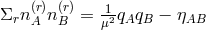 tangential to the 4-dimensional surface
 , i.e.,
 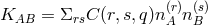 . The
. The  were assumed to be self-adjoined
operators with commutation relations
were assumed to be self-adjoined
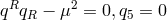
operators with commutation relations ![[C ∗(ij,q),C(lm, q′)] = (δim δjl + δjmδil − &tidle;bδijδlm )δ (qRqR − μ2)](article2936x.gif) .
.  is
a new numerical parameter. The commutation relations for the fields then were calculated to have the form:
is
a new numerical parameter. The commutation relations for the fields then were calculated to have the form:
![[ϕ (x ),ϕ (x ′)] = (P P + P P − &tidle;bP P )𝒟(x − x ′) (539 ) AB CD AC BD AD BC AB CD](article2938x.gif)
 and the Pauli–Jordan distribution
  . (539*) translated into
and is independent of a if
. (539*) translated into
and is independent of a if ![′ [kAB (x),kCD (x )] = 3 − d 2 3 ∂4 ′ (PAC PBD + PADPBC − -----PABPCD − -d (-4---A---B---C---D + ηAB ηCD )𝒟(x − x ) (540 ) 6 9 μ ∂x ∂x ∂x ∂x](article2941x.gif)
 holds. The paper of S. Lederer discussed here in some
detail is one midway in a series of contributions to the quantization of the linearized Jordan–Thiry theory
begun with the publications of C. Morette-Dewitt & B. Dewitt, [448, 449], continued by Ph. Droz-Vincent
[129, 128*],289
and among others by A. Capella [72] and Cl. Roche [511].
holds. The paper of S. Lederer discussed here in some
detail is one midway in a series of contributions to the quantization of the linearized Jordan–Thiry theory
begun with the publications of C. Morette-Dewitt & B. Dewitt, [448, 449], continued by Ph. Droz-Vincent
[129, 128*],289
and among others by A. Capella [72] and Cl. Roche [511].
These papers differ in their assumptions; e.g., Droz-Vincent worked with the traceless quantity
 ; for
; for  , and thus for
  his results agree with those of S. Lederer.
In his earlier paper, A. Capella had taken
his results agree with those of S. Lederer.
In his earlier paper, A. Capella had taken  , and
, and  . Claude Roche applied the methods
of Ph. Droz-Vincent to the case of mass zero fields and quantized the gravitational and the electromagnetic
fields simultaneously.
. Claude Roche applied the methods
of Ph. Droz-Vincent to the case of mass zero fields and quantized the gravitational and the electromagnetic
fields simultaneously.
16.3 Linear theory and spin-1/2-particles
With the progress in elementary particle theory, group theory became instrumental for the idea of
unification. J.-M. Souriau was one of those whose research followed this line. His unitary field theory
started with a relativity principle in 5-dimensional space the underlying group of which he called “the
5-dimensional Lorentz group” but essentially was a product of the 4-dimensional Poincaré group
with the group  of 2-dimensional real orthogonal matrices. For its infinitesimal generator
 holds wherefrom he introduced the integer
  by
by  . He interpreted
 as the electric charge of a particle and brought charge conjugation (
 ) and
antiparticles into his formalism [582]. Souriau also asked whether quantum electrodynamics could
be treated in the framework of Thiry’s theory, but for obvious reasons only looked at wave
equations for spin-0 and spin-1/2 particles. As a result, he claimed to have shown the existence of
two neutrinos of opposite chirality and maximum violation of parity in
) and
antiparticles into his formalism [582]. Souriau also asked whether quantum electrodynamics could
be treated in the framework of Thiry’s theory, but for obvious reasons only looked at wave
equations for spin-0 and spin-1/2 particles. As a result, he claimed to have shown the existence of
two neutrinos of opposite chirality and maximum violation of parity in  -decay [583]. By
comparing the (inhomogeneous) 5-dimensional wave equation for solutions of the form of the
Fourier series
-decay [583]. By
comparing the (inhomogeneous) 5-dimensional wave equation for solutions of the form of the
Fourier series  with the Klein–Gordon equation in an
electromagnetic field, he obtained the spectrum of eigenvalues for charge
with the Klein–Gordon equation in an
electromagnetic field, he obtained the spectrum of eigenvalues for charge  and mass
  :
:
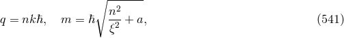
 ,
,  is the gravitational constant in Einstein’s equations, and
  the
“mass”-term of the 5-dimensional wave equation, i.e., a free parameter.
the
“mass”-term of the 5-dimensional wave equation, i.e., a free parameter.  is the scalar field:
  .
For
.
For  ,
,  is of the order of magnitude
  . Souriau also rewrote Dirac’s equation in
flat space-time of five dimensions as an equation in quaternion space for 2 two-component neutrinos. His
interpretation was that the electromagnetic interaction of fermions and bosons has a geometrical origin. The
charge spectrum is the same as for spin-0 particles except that the constant
. Souriau also rewrote Dirac’s equation in
flat space-time of five dimensions as an equation in quaternion space for 2 two-component neutrinos. His
interpretation was that the electromagnetic interaction of fermions and bosons has a geometrical origin. The
charge spectrum is the same as for spin-0 particles except that the constant  in (541*) is replaced by
 .
.
O. Costa de Beauregard applied the linear approximation of Souriau’s theory for a field variable  to describe the equations for a spin-1/2 particle coupled to the photon-graviton system. He obtained the
equation
to describe the equations for a spin-1/2 particle coupled to the photon-graviton system. He obtained the
equation  , where the wave function
  again
depends on the coordinate
again
depends on the coordinate  via
via  ; as before,
  is the coupling constant in Einstein’s field
equations. Comparison with electrodynamics led to the identification
is the coupling constant in Einstein’s field
equations. Comparison with electrodynamics led to the identification  with
with  the electric
charge. Costa de Beauregard also suggested an experimental test of the theory with macroscopic bodies
[91].
the electric
charge. Costa de Beauregard also suggested an experimental test of the theory with macroscopic bodies
[91].
16.4 Quantization of Einstein–Schrödinger theory?
Together with efforts at the quantization of the gravitational field as described by general relativity, also
attempts at using Einstein–Schrödinger type unified theories instead began. Linearization
around Minkowski space was an obvious possibility. But then the argument that the cosmological
constant had appeared in some UFTs (Schrödinger) lead to an attempt at quantization in curved
space-time. In the course of his research, A. Lichnerowicz developed a method of expanding
the field equations around both a metric and a connection which are solutions of equations
describing a fixed geometric backgrond [375*]. Quantization then was applied to the quantities varied
(semi-classical approximation). The theory was called “theory of the varied field” by Tonnelat [641*],
p. 441).290
Lichnerowicz determined the “commutators corresponding to vector meson and to an electromagnetic field
(spin 1) on one hand and to a microscopic gravitational field (spin 2, mass 0) on the other hand […] in terms
of propagators” [378]. The linearization was obtained by looking at field equations for the varied metric and
connection. Let  be such a variation of the metric
  and
and  a variation of
the connection
a variation of
the connection  . It is straightforward to show that the variation of the Ricci tensor is
 , where the covariant derivative is taken with regard to the
connection formed from
, where the covariant derivative is taken with regard to the
connection formed from  . Also,
  . Ph. Droz-Vincent then looked at
field equations for a connection with vanishing vector torsion and with Einstein’s compatibility equation
(30*) varied, i.e.,
. Ph. Droz-Vincent then looked at
field equations for a connection with vanishing vector torsion and with Einstein’s compatibility equation
(30*) varied, i.e.,  :
:

 and arbitrary
  [131].291
The Riemannian metric which is varied solves
[131].291
The Riemannian metric which is varied solves  (Einstein space). Droz-Vincent showed that
the variation
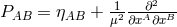
(Einstein space). Droz-Vincent showed that
the variation  must satisfy the equations:
where
must satisfy the equations:
where ![∇rΨ = 0 , (543 ) [rj] (Δ + 2λ)Ψ (ij) = ∇ikj + ∇jki, (544 ) 8 (D + 2 λ)Ψ[ij] = -∂ [iδΓ j], (545 ) 3](article2994x.gif)
 is a differential operator different from the Laplacian
  for the Riemannian metric
introduced by Lichnerowicz ([375], p. 28) such that
for the Riemannian metric
introduced by Lichnerowicz ([375], p. 28) such that  .
.  is defined by
 (indices moved with
  ). Equation (543*) follows from the vanishing of vector
torsion.
). Equation (543*) follows from the vanishing of vector
torsion.
Difficulties arose with the skew-symmetric part of the varied metric. Quantization must be performed such as to be compatible with this condition. The commutators sugested by Lichnerowicz were not compatible with (397*). Droz-Vincent refrained from following up the scheme because:
“The endeavour to establish such a program is, to be sure, a bit premature in view of the
missing secure physical interpretation of the objects to be quantized.”292
Ph. Droz-Vincent sketched how to write down Poisson brackets and commutation relations for the
Einstein–Schrödinger theory also in the framework of the “theory of the varied field” ([130]. In general, the
main obstacle for quantization is formed by the constraint equations, once the field equations are split into
time-evolution equations and constraint equations. Droz-Vincent distinguished between proper and
improper dynamical variables. The system  , where
  signifies covariant derivation
with respect to the star connection (27*), led to 5 constraint equations containing only proper variables
arising from general covariance and
signifies covariant derivation
with respect to the star connection (27*), led to 5 constraint equations containing only proper variables
arising from general covariance and  -invariance. By destroying
  -invariance via a term
 , one of the constraints can be eliminated. The Poisson brackets formed from these
constraints were well defined but did not vanish. This was incompatible with the field equations. By
introducing a non-dynamical timelike vector field and its first derivatives into the Lagrangian,
Ph. Droz-Vincent could circumvent this problem. The physical interpretation was left open
[133, 135]. In a further paper, he succeeded in finding linear combinations of the constraints whose
Poisson brackets are zero modulo the constraints themselves and thus acceptable for quantization
[136].
, one of the constraints can be eliminated. The Poisson brackets formed from these
constraints were well defined but did not vanish. This was incompatible with the field equations. By
introducing a non-dynamical timelike vector field and its first derivatives into the Lagrangian,
Ph. Droz-Vincent could circumvent this problem. The physical interpretation was left open
[133, 135]. In a further paper, he succeeded in finding linear combinations of the constraints whose
Poisson brackets are zero modulo the constraints themselves and thus acceptable for quantization
[136].
 |
 |
 |
Living Rev. Relativity, 17 (2014), 5, doi:10.12942/lrr-2014-5, URL (accessed <date>): http://www.livingreviews.org/lrr-2014-5.
 This work is licensed under a Creative Commons License.
© The author(s), except where otherwise noted.
This work is licensed under a Creative Commons License.
© The author(s), except where otherwise noted.