13 Research in other English Speaking Countries
13.1 England and elsewhere
We have met the work of W. B. Bonnor of the University of Liverpool on UFT already before.
After having investigated exact solutions of the “weak” and “strong” field equations, he set
up his own by adding the term  to Einstein’s Lagrangian of UFT [34]. They
are:254
to Einstein’s Lagrangian of UFT [34]. They
are:254
![gi+k−||l = 0, (464 ) S = 0, (465 ) i HKer + p2U = 0, (466 ) − (ik) (ij) Her Her Her K [ik],l + K [kl],i + K [li],k + p2(U [ik],l + U [kl],i + U [li],k) = 0, (467 ) − − −](article2486x.gif)
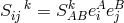
![[rs] 1 [rs] Uij = g[ij] − g girgjs + -g grsgij. (468 ) 2](article2487x.gif)
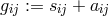
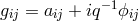
The assignment of  to the gravitational potentials and of
 ![g[ij]](article2489x.gif) to the electromagnetic field was
upheld while the electric current became defined as
to the electromagnetic field was
upheld while the electric current became defined as ![Jijk = g{[ij],k}](article2490x.gif) .
.
A linearization 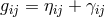 of Bonnor’s field equations up to the first order in
  led to:
![γ[is],s = 0, γ(is),sk + γ(ks),si − γss,ki = 0, (469 ) γ = − 4p2γ . (470 ) {[ik],l},ss {[ik],l}](article2493x.gif)
![Jijk = γ{[ij],k}](article2494x.gif) such that the previous equation
looked like
such that the previous equation
looked like  . For a spherically symmetric particle at rest with radial coordinate
  ,
Bonnor obtained
where
,
Bonnor obtained
where 
 is the charge density. For
  and
and  for
for  , the charge density will be
restricted255
to
, the charge density will be
restricted255
to  . As M.-A. Tonnelat remarked, Bonnor’s strategy was simply to add a term leading
to Maxwell’s energy-momentum-stress tensor ([634], p. 919). Abrol & Mishra later re-wrote
Bonnor’s field equations with help of the connections defined in (51*) and (52*) of Section 2.2.3
[2].
. As M.-A. Tonnelat remarked, Bonnor’s strategy was simply to add a term leading
to Maxwell’s energy-momentum-stress tensor ([634], p. 919). Abrol & Mishra later re-wrote
Bonnor’s field equations with help of the connections defined in (51*) and (52*) of Section 2.2.3
[2].
In Trinity College, Cambridge, UK, in the mid-1950s research on UFT was carried out by John
Moffat as part of his doctoral thesis. It was based on a complex metric in (real) space-time:
 with real
  , imaginary
  , and
, and  . Correspondingly, the symmetrical linear
connection
. Correspondingly, the symmetrical linear
connection  split into a real connection part
  and an imaginary valued tensor
 .256
His approach to UFT then differed considerably from Einstein’s. In place of (16*) of Section 2.1.1 now
.256
His approach to UFT then differed considerably from Einstein’s. In place of (16*) of Section 2.1.1 now


![Γ s [δk+ ∗skrars] = HL j ij s ik](article2514x.gif) except that the imaginary
except that the imaginary  is entering on both sides; cf. Eqs. (8) – (10),
p. 624 in [439*]. It seems that Moffat did know neither Einstein’s papers concerning UFT with
a complex metric [147, 148] (see Section 7.2) nor Hattori’s connection. This is unsurprising
in view of his thesis advisors F. Hoyle and A. Salam which were not known as specialists in
UFT.
With these complex valued mathematical objects, Moffat now built a “generalization of gravitation theory” [440*]
with the explicit purpose to find a theory yielding the correct equations of motion for charged particles (Lorentz
force).257
Now,
is entering on both sides; cf. Eqs. (8) – (10),
p. 624 in [439*]. It seems that Moffat did know neither Einstein’s papers concerning UFT with
a complex metric [147, 148] (see Section 7.2) nor Hattori’s connection. This is unsurprising
in view of his thesis advisors F. Hoyle and A. Salam which were not known as specialists in
UFT.
With these complex valued mathematical objects, Moffat now built a “generalization of gravitation theory” [440*]
with the explicit purpose to find a theory yielding the correct equations of motion for charged particles (Lorentz
force).257
Now,  and
and  . As a real Lagrangian, Moffat chose:
where presumably
. As a real Lagrangian, Moffat chose:
where presumably ![√ --- rs rs ˆ ℒ= − g[∗g ∗ Rrs + ˆg Rrs], (474 )](article2520x.gif)
 is defined by the decomposition of the inverse
  of
of  with
with  , i.e.,
 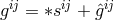 , although this relationship is not written down. His
Ricci-tensors to be added to the list in Section 2.3.2 are the real and complex parts of
, although this relationship is not written down. His
Ricci-tensors to be added to the list in Section 2.3.2 are the real and complex parts of  W. Pauli’s objection in its strict sense still applies in spite of the Lagrangian being a sum of irreducible
terms.
W. Pauli’s objection in its strict sense still applies in spite of the Lagrangian being a sum of irreducible
terms.

For the field variables  , in empty space the field equations following from (474*) are

 with “the complex-symmetric source
term”
with “the complex-symmetric source
term”  ,
,  the Newtonian gravitational constant. According to Moffat: “The real
tensor
the Newtonian gravitational constant. According to Moffat: “The real
tensor  represents the energy-momentum of matter, while
  is the charge-current
distribution.” A weak-field-approximation
is the charge-current
distribution.” A weak-field-approximation 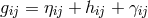 with real
  and imaginary
  is then carried through. In 1st approximation, the wave equation
  resulted
where
resulted
where  and
and  . For slowly moving point particles and weak fields,
Maxwell–Lorentz electrodynamics was reached. After an application of the EIH-approximation
scheme up to the 6th approximation omitting cross tems between charge and mass, Moffat
concluded:258
“we have derived from the field equations the full Lorentz equations of motion with relativistic corrections
for charged particles moving in weak and quasi-stationary electromagnetic fields.” In a note added in proof
he claimed that his method of winning the equations of motion was valid also for “quickly varying fields and
fast moving particle” ([440*], p. 487). In place of the Reissner–Nordström metric, he obtained as a static
centrally symmetric metric [441*]:
. For slowly moving point particles and weak fields,
Maxwell–Lorentz electrodynamics was reached. After an application of the EIH-approximation
scheme up to the 6th approximation omitting cross tems between charge and mass, Moffat
concluded:258
“we have derived from the field equations the full Lorentz equations of motion with relativistic corrections
for charged particles moving in weak and quasi-stationary electromagnetic fields.” In a note added in proof
he claimed that his method of winning the equations of motion was valid also for “quickly varying fields and
fast moving particle” ([440*], p. 487). In place of the Reissner–Nordström metric, he obtained as a static
centrally symmetric metric [441*]:
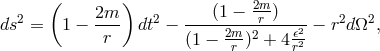
 denotes the electric charge. Upon criticism by W. H. McCrea and W. B. Bonnor, Moffat
included the “dipole procedure” of Einstein and Infeld in his derivation of the equations of motion [442].
R. P. Kerr found that the field equations (477*), together with the boundary conditions at spacelike infinity,
are not sufficient to determine the spherically symmetric solution. This holds even when four coordinate
conditions are added [324].
denotes the electric charge. Upon criticism by W. H. McCrea and W. B. Bonnor, Moffat
included the “dipole procedure” of Einstein and Infeld in his derivation of the equations of motion [442].
R. P. Kerr found that the field equations (477*), together with the boundary conditions at spacelike infinity,
are not sufficient to determine the spherically symmetric solution. This holds even when four coordinate
conditions are added [324].
In the 1950s, the difficulty with the infinities appearing in quantum field theory in calculations of higher order terms (perturbation theory) had been overcome by Feynman, Schwinger, Tomonoga and Dyson by renormalization schemes. Nevertheless, in 1952, Behram Kursunŏglu as a PhD student in Cambridge, UK, expressed the opinion,
“[…] that a correct and unified quantum theory of fields, without the need of the so-called renormalization of some physical constants, can be reached only through a complete classical field theory that does not exclude gravitational phenomena.” ([343*], p. 1396.)
![√ --- ℒ= ˆgrsRrs − 2p2[ − b − √ − g-], (478 )](article2543x.gif)
 and
and  is the inverse to the symmetric part
  of the asymmetric metric
 .259
I assume that his Ricci tensor
.259
I assume that his Ricci tensor  is the same as the one used by Einstein in [149], i.e.,
  .
.
By an approximation around Euclidean space 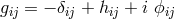 which neglected the squares of
 , the cubes of
  , and interaction terms between
  , Kursunŏglu obtained the following
results:
, Kursunŏglu obtained the following
results:
![bij = − δij + hij − T ′, T ′= 1δijΣr,s(ϕrsϕrs) − Σr(ϕirϕjr), (479 ) ij ij 4 1- ∂sfsi = Ji, Ilrs = Σt(𝜖lrstJt), fij = − 2 Σk,l(𝜖ijklϕkl) = ∂iAj − ∂jAi, (480 ) 1 1 ( 1 ) --□hij + --[δijΣr(JrJr) − JiJj] + Σr,s(∂rϕjs∂sϕir) + ∂i∂j -Σr,s(frsfrs) 2 2 4 1- 2 + 2 [Σr (firJjr) + Σr(fjrJir) − δijΣr,s(frsJrs)] = p Tij, (481 )](article2556x.gif)
![Jij = 2∂ [iJj]](article2557x.gif) , and
, and  . Both
  and
and  are identified with the electromagnetic field:

 with the Einstein field equations of general relativity, the relation
 with the gravitational constant
  ensued. Kursunŏglu then put the focus on
the equation for the electrical current density derived from (302*) after a lengthy calculation:
where
ensued. Kursunŏglu then put the focus on
the equation for the electrical current density derived from (302*) after a lengthy calculation:
where 
 is a function describing the interaction terms; it consists of 11 products of
  with
with  or
or
 or
or  (and up to their 2nd derivatives). The r.h.s. of (482*) then was summarily replaced by
![|E | = e2[1 − e−κr − κre− κr] − r](article2572x.gif) .
Kursunŏglu concluded that UFT “describes the charge density of an elementary particle as a
short range field. It is not possible to measure the effects of an electron “radius”
.
Kursunŏglu concluded that UFT “describes the charge density of an elementary particle as a
short range field. It is not possible to measure the effects of an electron “radius”  by
having two electrons collide with an energy of the order of
by
having two electrons collide with an energy of the order of  . Quantum theoretically the
wavelength corresponding to this energy is
. Quantum theoretically the
wavelength corresponding to this energy is  , which is much larger than
  .” ([343] ,
p. 1375.)
.” ([343] ,
p. 1375.)
As to the equations of motion, Kursunŏglu assumed that (30*) is satisfied and, after some
approximations, claimed to have obtained the Lorentz equation, in lowest order with an inertial mass
 (cf. his equations (7.8) – (7.10)); thus according to him, inertial mass is of purely
electromagnetic nature: no charge – no mass! Whether this result amounted to an advance, or to a regress
toward the beginning of the 20th century is left open.
(cf. his equations (7.8) – (7.10)); thus according to him, inertial mass is of purely
electromagnetic nature: no charge – no mass! Whether this result amounted to an advance, or to a regress
toward the beginning of the 20th century is left open.
In a short note with G. Rickayzen, Kursunŏglu pointed out that the Born–Infeld non-linear
electrodynamics followed from his “version of Einstein’s generalized theory of gravitation” in the limit
 . In the note, a Lagrangian differing from (478*) appeared:
![2 rs 2 2 √ --- √ --- 2p ℒ= ˆg (Rrs − ip Brs) + 2p [ − b − − g ], (483 )](article2579x.gif)
![Brs = 2∂[rBs]](article2580x.gif) is an auxiliary field variable [509].
is an auxiliary field variable [509].
G. Stephenson from the University College in London altered Einstein’s field
equation as given in Appendix II of the 4th London edition of The Meaning of
Relativity260
by replacing the constraint on vector torsion  by
by  with constant
  , and by introducing
a vector-potential
, and by introducing
a vector-potential  for the electromagnetic field tensor
  [588]. His split of (30*) for the symmetric
part coincided with Tonnelat’s (363*), but differed for the skew-symmetric part from her (362*) of
Section 10.2.3. The missing term is involved in Stephenson’s derivation of his result: Dirac’s
electrodynamics
[588]. His split of (30*) for the symmetric
part coincided with Tonnelat’s (363*), but differed for the skew-symmetric part from her (362*) of
Section 10.2.3. The missing term is involved in Stephenson’s derivation of his result: Dirac’s
electrodynamics  . Hence the validity of this result is unclear.
A year later, Stephenson delved deeper into affine UFT [589]. We quote from the review written by one
of the opinion leaders, V. Hlavatý, for the Mathematical Reviews [ MR0068357]:
“The Einstein paper contains three separate sections. In the first section the author
expresses the symmetric part  of the unified field connection
  by
means of its skew symmetric part
by
means of its skew symmetric part ![ν ν Sλμ = Γ[λμ]](article2589x.gif) and vice versa. Then he identifies
the electromagnetic field with
and vice versa. Then he identifies
the electromagnetic field with ![k λμ = g[λμ]](article2590x.gif) and imposes on it the first set of Maxwell
conditions
and imposes on it the first set of Maxwell
conditions
![∂[ωk μλ] = 0.](article2591x.gif)
The second set of Maxwell conditions is equivalent to the Einstein condition  .
However, according to the author, there appears to be no definite reason for imposing
the additional condition (1). In the second part the author considers Einstein’s condition
.
However, according to the author, there appears to be no definite reason for imposing
the additional condition (1). In the second part the author considers Einstein’s condition
![R [μλ] = 2 ∂[μX λ]](article2593x.gif)
coupled with
![α R [μλ] = − D αSμλ](article2594x.gif)
(where  denotes the covariant derivative with respect to
  ). Hence
![S νμλ = 2X [μδνλ] + T νμλ,](article2597x.gif)
where ![ν ν Tμλ = T [μλ]](article2598x.gif) is a solution of
is a solution of

Therefore  is equivalent to
and the field equations reduce to 16 equations (4) and  . In the third part the
author considers all possibilities of defining
. In the third part the
author considers all possibilities of defining  by means of the derivatives of
  with all possible combinations of Einstein’s signs
  ,
,  ,
,  . He concludes
that in both cases (i.e. for real or complex
. He concludes
that in both cases (i.e. for real or complex  ) only the
  derivation leads to a
connection
derivation leads to a
connection  without imposing severe restrictions on
  .”
.”
13.1.1 Unified field theory and classical spin
Each of the three scientists described above introduced a new twist into UFT within the framework of – real
or complex – mixed geometry in order to cure deficiencies of Einstein’s theory (weak field equations).
Astonishingly, D. Sciama at first applied the full
machinery of metric affine geometry in order to merely describe the gravitational field. His
main motive was “the possibility that our material system has intrinsic angular momentum or
spin”, and that to take this into account “can be done without using quantum theory” ([565*],
p. 74). The latter remark referred to the concept of a classical spin (point) particle characterized
by mass and an antisymmetric “spin”-tensor  . Much earlier, Mathisson
(1897 – 1940) [392, 391, 393], Weyssenhoff (1889 – 1972) [695, 694] and Costa de Beauregard
(1911 – 2007) [87], had investigated this concept. For a historical note cf. [584]. Sciama did not give a
reference to C. de Beauregard, who fifteen years earlier had pointed out that both sides of
Einstein’s field equations must become asymmetric if matter with spin degrees of freedom is
generating the gravitational field. Thus an asymmetric Ricci tensor was needed. It also had
been established that the deviation from geodesic motion of particles with charge or spin is
determined by a direct coupling to curvature and the electromagnetic field
. Much earlier, Mathisson
(1897 – 1940) [392, 391, 393], Weyssenhoff (1889 – 1972) [695, 694] and Costa de Beauregard
(1911 – 2007) [87], had investigated this concept. For a historical note cf. [584]. Sciama did not give a
reference to C. de Beauregard, who fifteen years earlier had pointed out that both sides of
Einstein’s field equations must become asymmetric if matter with spin degrees of freedom is
generating the gravitational field. Thus an asymmetric Ricci tensor was needed. It also had
been established that the deviation from geodesic motion of particles with charge or spin is
determined by a direct coupling to curvature and the electromagnetic field  or,
analogously, curvature and the classical spin tensor
or,
analogously, curvature and the classical spin tensor  . The energy-momentum tensor of
a spin-fluid (Cosserat continuum), discussed in materials science, is skew-symmetric. What
Sciama attempted was to geometrize the spin-tensor considered before just as another field in
space-time.
Because he insisted on physical space as being described by Riemannian geometry, he had to
cope with two geometries, the one with the full asymmetric metric
. The energy-momentum tensor of
a spin-fluid (Cosserat continuum), discussed in materials science, is skew-symmetric. What
Sciama attempted was to geometrize the spin-tensor considered before just as another field in
space-time.
Because he insisted on physical space as being described by Riemannian geometry, he had to
cope with two geometries, the one with the full asymmetric metric  , and space-time with
metric
, and space-time with
metric  where
where  , an attribution which we have seen before in the work of
Lichnerowicz. This implied that spinless particles moved on geodesics of the metric
, an attribution which we have seen before in the work of
Lichnerowicz. This implied that spinless particles moved on geodesics of the metric  , even if the
gravitational field is generated by a massive spinning source, while spinning particles move on
non-geodesic orbits determined by the non-symmetric connection. Sciama’s field equations were:
, even if the
gravitational field is generated by a massive spinning source, while spinning particles move on
non-geodesic orbits determined by the non-symmetric connection. Sciama’s field equations were:
![dui dg[il] ----= ul----. (487 ) ds ds](article2620x.gif)
Perhaps, Sciama had convinced himself that mixed geometry was too rich in geometrical
objects for the description of just one, the gravitational interaction. In any case, in his next
five papers in which he pursued the relation between (classical) spin and geometry, he went
into UFT proper [565*]. He first dealt with the electromagnetic field which he identified with
an expression looking like homothetic curvature: 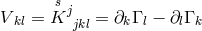 . However,
here
. However,
here ![r Γ k := L [kr] = Sk](article2622x.gif) In order to reach this result he had introduced a complex tetrad
field261
and defined a complex curvature tensor
In order to reach this result he had introduced a complex tetrad
field261
and defined a complex curvature tensor  skew-symmetric in one pair of its indices and
“skew-Hermitian” in the other. In analogy to Weyl’s second attempt at gauge theory [692], he arrived at
the trace of the tetrad-connection as his “gauge-potential” without naming it such. He also
introduced a “principle of minimal coupling” as an equivalent to the “equivalence principle” of
general relativity: matter must not directly couple to curvature in the Lagrangian of a theory.
M.-A. Tonnelat and L. Bouche [646] then showed that Sciama’s non-symmetric theory of the pure
gravitational field [565*] “implies that the streamlines of a perfect fluid
skew-symmetric in one pair of its indices and
“skew-Hermitian” in the other. In analogy to Weyl’s second attempt at gauge theory [692], he arrived at
the trace of the tetrad-connection as his “gauge-potential” without naming it such. He also
introduced a “principle of minimal coupling” as an equivalent to the “equivalence principle” of
general relativity: matter must not directly couple to curvature in the Lagrangian of a theory.
M.-A. Tonnelat and L. Bouche [646] then showed that Sciama’s non-symmetric theory of the pure
gravitational field [565*] “implies that the streamlines of a perfect fluid  are
geodesics of the Riemannian space with metric
are
geodesics of the Riemannian space with metric  . These streamlines are not geodesics of the
metric
. These streamlines are not geodesics of the
metric  , but deviate from them by an amount which, in first approximation, agrees with a
heuristic formula occurring in Costa de Beauregard’s theory of the gravitational effects of spin
[89]”.262
, but deviate from them by an amount which, in first approximation, agrees with a
heuristic formula occurring in Costa de Beauregard’s theory of the gravitational effects of spin
[89]”.262
In his next paper, Sciama described his endeavour of geometrizing classical spin within a general conceptual framework for unified field theory. His opening words made clear that he found it worthwhile to investigate UFT:
“The majority of physicists considers with some reserve unified field theory. In this article,
my intention is to suggest that such a reserve is not justified. I will not explain or defend a
particular theory but rather discuss the physical importance of non-Riemannian theories
in general.” ([566], p. 1.)263
Sciama’s main new idea was that the holonomy group plays an important rôle with its subgroup,
Weyl’s  , leading to electrodynamics, and another subgroup, the Lorentz group, leading to the spin
connection. Although he gave the paper of Yang & Mills [712] as a reference, he obviously did not
know Utiyama’s use of the Lorentz group as a “gauge group” for the gravitational field [661].
C. de Beauregard‘s reaction to Sciama’s paper was immediate: he agreed with him as to the
importance of embedding spin into geometry but did not like the two geometries introduced in
[565]. He also suggested an experiment for measuring effects of (classical) spin in space-time
[88].
, leading to electrodynamics, and another subgroup, the Lorentz group, leading to the spin
connection. Although he gave the paper of Yang & Mills [712] as a reference, he obviously did not
know Utiyama’s use of the Lorentz group as a “gauge group” for the gravitational field [661].
C. de Beauregard‘s reaction to Sciama’s paper was immediate: he agreed with him as to the
importance of embedding spin into geometry but did not like the two geometries introduced in
[565]. He also suggested an experiment for measuring effects of (classical) spin in space-time
[88].
In another paper of the same year, Sciama opted for a different identification of classical spin
with geometrical structure: the skew-symmetric part of the connection no longer was solely
connected with the electromagnetic field but with the spin angular moment of matter [567*]. By
introducing a field  like a (classical) Dirac spinor, he defined the spin-flux as
  where
where  is a fitting representation of the Lorentz group. The indices
  are tetrad-indices (real tetrad
  ), introduced by
  . Seemingly, at that point
Sciama had not known Cartan’s calculus with differential forms and reproduced the calculation of
tetrad connection and curvature tensor in a somewhat clumsy notation. The result of interest is:
. Seemingly, at that point
Sciama had not known Cartan’s calculus with differential forms and reproduced the calculation of
tetrad connection and curvature tensor in a somewhat clumsy notation. The result of interest is:
![L k= S k+ δkS (488 ) [ij] ij [i j]](article2634x.gif)
 . Use of a complex tetrad allowed him to define the electromagnetic field as
before. At the time, he must have had an interaction with T. W. B. Kibble who’s paper on
“Lorentz Invariance and the Gravitational Field” introduced the Poincaré group as a gauge
group264
[325]. Sciama’s next paper did not introduce new ideas but presented his calculations and interpretation in
further detail [568]. Two years later, when the ideas of Yang & Mills and Utiyama finally had been accepted
by the community as important for field theory, Sciama for the first time named his way of introducing the
skew-symmetric part of the connection “the now fashionable ‘gauge trick’ ” ([569*], p. 465, 466). His
interpretation of UFT had changed entirely:
. Use of a complex tetrad allowed him to define the electromagnetic field as
before. At the time, he must have had an interaction with T. W. B. Kibble who’s paper on
“Lorentz Invariance and the Gravitational Field” introduced the Poincaré group as a gauge
group264
[325]. Sciama’s next paper did not introduce new ideas but presented his calculations and interpretation in
further detail [568]. Two years later, when the ideas of Yang & Mills and Utiyama finally had been accepted
by the community as important for field theory, Sciama for the first time named his way of introducing the
skew-symmetric part of the connection “the now fashionable ‘gauge trick’ ” ([569*], p. 465, 466). His
interpretation of UFT had changed entirely:
“We may note in passing that the result (7) [here Eq. (488*)] suggests that unified field theories based on a non-symmetric connection have nothing to do with electromagnetism.” ([569], p. 467)
C. de Beauregard had expressed this opinion three years earlier; moreover his doubts had been directed against the “unified theory of Einstein–Schrödinger-type” in total [90]. In the 1960s, the subject of classical spin and gravitation was taken up by F. W. Hehl [245] and developed into “Poincaré gauge theory” with his collaborators [246].
13.2 Australia
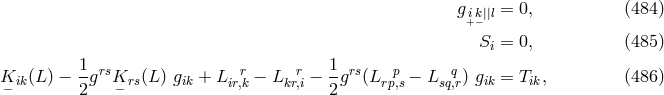
H. A. Buchdahl
in Tasmania, Australia, added a further definition for the electrical current, i.e., ![ˆjk = ˆg[kl] ,l](article2636x.gif) .
Then, in linear approximation, from (211*), the unacceptable restriction
.
Then, in linear approximation, from (211*), the unacceptable restriction  followed. In
order to remedy this defect, Buchdahl suggested another set of field equations which, with an
appropriate Lagrangian, did not imply any restriction on the thus defined electric current [64]:
followed. In
order to remedy this defect, Buchdahl suggested another set of field equations which, with an
appropriate Lagrangian, did not imply any restriction on the thus defined electric current [64]:
![+ik− ˆk [kl] ˆg ∥l = 0, g[ij] = ∂[kAi], j = ˆg ,l, (489 ) Bˆ(ij) = 0, ˆB[il]= 0, (490 ) ,l](article2638x.gif)
 ,
,  an arbitrary vector. Unfortunately, from a linear approximation in which only
the antisymmetric part of the metric is considered to be weak, an unacceptable result followed:
“Consequently, if one wishes to maintain an unrestricted current vector is would seem that the introduction
of a vector potential
an arbitrary vector. Unfortunately, from a linear approximation in which only
the antisymmetric part of the metric is considered to be weak, an unacceptable result followed:
“Consequently, if one wishes to maintain an unrestricted current vector is would seem that the introduction
of a vector potential  in the manner above must be abandoned.” ([65*], p. 1145.) With the asymmetric
metric
in the manner above must be abandoned.” ([65*], p. 1145.) With the asymmetric
metric  having gauge weight
  the determinant
  is of gauge weight
  for dimension
  of the manifold ).
Buchdahl then set out to build a gauge-invariant unified field theory by starting from Weyl space with
symmetric metric
of the manifold ).
Buchdahl then set out to build a gauge-invariant unified field theory by starting from Weyl space with
symmetric metric  and linear connection
  . The gauge transformation is
given by
. The gauge transformation is
given by  . Tensor densities now have both a coordinate weight
 [cf. (21*) of Section 2.1.1], and a gauge weight
  defined via the covariant derivative by:
([65], p. 90). As a gauge-invariant curvature tensor and its contractions were used, the curvature scalar
defined via the covariant derivative by:
([65], p. 90). As a gauge-invariant curvature tensor and its contractions were used, the curvature scalar 
 then is of gauge weight
  . Consequently, a gauge-invariant Lagrangian density must contain terms
quadratic in curvature like
. Consequently, a gauge-invariant Lagrangian density must contain terms
quadratic in curvature like  . Buchdahl used the gauge-invariant Hermitian Ricci tensor
  in
Eq. (73*) of Section 2.3.2, and the field equations [66*]:
Under scrutiny and by use of approximation methods and boundary conditions at (spatial) infinity, it
turned out, according to H. A. Buchdahl, that these equations very likely did not have acceptable physical
solutions ([66], p. 264). In view of the non-acceptance of Weyl’s original gauge theory of the gravitational
and electromagnetic fields, it is not surprising that Buchdahl’s gauge-invariant UFT did not lead to much
further research. One sequel was Mishra’s paper [436] in which an exact solution in place of Buchdahl’s
approximate one for weak fields is claimed; closer inspection shows that it is only implicitly given
(cf. Eq. (3.1), p. 84).
in
Eq. (73*) of Section 2.3.2, and the field equations [66*]:
Under scrutiny and by use of approximation methods and boundary conditions at (spatial) infinity, it
turned out, according to H. A. Buchdahl, that these equations very likely did not have acceptable physical
solutions ([66], p. 264). In view of the non-acceptance of Weyl’s original gauge theory of the gravitational
and electromagnetic fields, it is not surprising that Buchdahl’s gauge-invariant UFT did not lead to much
further research. One sequel was Mishra’s paper [436] in which an exact solution in place of Buchdahl’s
approximate one for weak fields is claimed; closer inspection shows that it is only implicitly given
(cf. Eq. (3.1), p. 84).

13.3 India
In a short note, the Indian theoretician G. Bandyopadhyay considered an affine theory using two variational principles such as
Schrödinger [553] had sugested in 1946 [9]. Besides his Ricci tensor  corresponding to
  of
(55*) he used another one
of
(55*) he used another one  turning out to be equal to:
  . The two
Lagrangians used were
. The two
Lagrangians used were  . The resulting field equations were:


 by allowing all signatures (“indices of
inertia”) for the symmetric part
by allowing all signatures (“indices of
inertia”) for the symmetric part  of the asymmetric metric and by splitting Hlavatý’s third class into
two [432*]:
of the asymmetric metric and by splitting Hlavatý’s third class into
two [432*]:
 and
and  . He then studied the solutions of (30*) for all classes and signatures
and showed that for a Riemannian metric only the first two classes exist while for signature zero all four
classes are possible. He also set out to show that the solution of M.-A. Tonnelat (cf. Section 10.2.3) is valid
only for the first class [434]. The conditions for Eqs. (30*), or (448*) to have a unique solution or to have at
least one solution are derived and discussed in extenso in several further papers [431, 432, 346*]. Tonnelat’s
conditions (364*) are made more precise:
. He then studied the solutions of (30*) for all classes and signatures
and showed that for a Riemannian metric only the first two classes exist while for signature zero all four
classes are possible. He also set out to show that the solution of M.-A. Tonnelat (cf. Section 10.2.3) is valid
only for the first class [434]. The conditions for Eqs. (30*), or (448*) to have a unique solution or to have at
least one solution are derived and discussed in extenso in several further papers [431, 432, 346*]. Tonnelat’s
conditions (364*) are made more precise:  . Except
for re-deriving Tonnelat’s result for class 1 (cf. [346], Eqs. (1.29)e, (1.30), p. 223), and polishing up
Hlavatý’s results by the inclusion of some degenerate subcases, e.g., for
. Except
for re-deriving Tonnelat’s result for class 1 (cf. [346], Eqs. (1.29)e, (1.30), p. 223), and polishing up
Hlavatý’s results by the inclusion of some degenerate subcases, e.g., for  for
for  , no new mathematical ideas were introduced. Physics was not mentioned at all.
Also, Mishra contradicted Kichenassamy’s papers in which Tonnelat’s results had been upheld
contrary to criticism by Hlavatý [326, 327]. Like in Wrede’s paper, Mishra considered the
generalization of “the concepts of Einstein’s unified field theory to n-dimensional space” as
well and derived “some recurrence relations for different classes of
, no new mathematical ideas were introduced. Physics was not mentioned at all.
Also, Mishra contradicted Kichenassamy’s papers in which Tonnelat’s results had been upheld
contrary to criticism by Hlavatý [326, 327]. Like in Wrede’s paper, Mishra considered the
generalization of “the concepts of Einstein’s unified field theory to n-dimensional space” as
well and derived “some recurrence relations for different classes of  ” [435]. In another
paper with S. K. Kaul, Mishra generalized Veblen’s identities (71*) of Section 2.3.1 to mixed
geometry with asymmetric connection. The authors obtained 4 identities containing 8 terms
each and with a mixture of
” [435]. In another
paper with S. K. Kaul, Mishra generalized Veblen’s identities (71*) of Section 2.3.1 to mixed
geometry with asymmetric connection. The authors obtained 4 identities containing 8 terms
each and with a mixture of  -derivatives [323]. I have seen no further application within
UFT. From my point of view as a historian of physics, R. S. Mishra’s papers are exemplary for
estimable applied mathematics uncovering some of the structures of affine and/or mixed geometry
without leading to further progress in the physical comprehension of unified field theory (cf. also
[429, 296]).
The generation of exact solutions to the Einstein–Schrödinger theory became a fashionable topic in India since
the mid 1960s. Following a suggestion of G. Bandyopadhyay, R. Sarkar assumed the asymmetric metric to have the
form:265
with
-derivatives [323]. I have seen no further application within
UFT. From my point of view as a historian of physics, R. S. Mishra’s papers are exemplary for
estimable applied mathematics uncovering some of the structures of affine and/or mixed geometry
without leading to further progress in the physical comprehension of unified field theory (cf. also
[429, 296]).
The generation of exact solutions to the Einstein–Schrödinger theory became a fashionable topic in India since
the mid 1960s. Following a suggestion of G. Bandyopadhyay, R. Sarkar assumed the asymmetric metric to have the
form:265
with ![( ) ds2 = H (dx0 )2 + 2Idx [1dx0] + (dx1)2 + G (dx2)2 + (dx3 )2 (495 )](article2677x.gif)
 and
and  being functions of the single variable
  [526]. In Hlavatý’s classification, the
metric was of second class. In terms of physics, static, one-dimensional gravitational and electromagnetic
fields were described. The particular set of solutions obtained consisted of metric components with algebraic
functions of
[526]. In Hlavatý’s classification, the
metric was of second class. In terms of physics, static, one-dimensional gravitational and electromagnetic
fields were described. The particular set of solutions obtained consisted of metric components with algebraic
functions of  and
and  , and showed (coordinate?) singularities. As a physical
interpretation, Sarkar offered the analogue to a Newtonian gravitating infinite plane. The limit
, and showed (coordinate?) singularities. As a physical
interpretation, Sarkar offered the analogue to a Newtonian gravitating infinite plane. The limit  in the
metric components led back to Bandyopadhyay’s solution [7] referred to in Section 9.6.2 (with some
printing errors removed by Sarkar):
in the
metric components led back to Bandyopadhyay’s solution [7] referred to in Section 9.6.2 (with some
printing errors removed by Sarkar):
![√ - √ - 2 G = (k + 3- bx1)43, H = 1∕b(k + 3- bx1)− 23[a − ------d√------], I = √1- ------d√------- 4 4 (k + 3 bx1 )83 b (k + 3 bx1)53 4 4](article2684x.gif)
 .
.
In a sequel [527], Sarkar used the asymmetric metric:
where, again![2 0 2 [2 3] 1 2 ( 2 2 32) ds = H (dx ) + 2Kdx dx + (dx ) + G (dx ) + (dx ) , (496 )](article2686x.gif)
 are functions of
  . The solutions found are static and with coordinate
singularities. To give just one metrical component:
. The solutions found are static and with coordinate
singularities. To give just one metrical component:
![∘ --- − 1 2 2L −1 C1 H = M [C1 exp(μx ) + C2exp (− μx)]3 × exp[− -√-------tan ---exp(μx ) ] μ C1C2 C2](article2689x.gif)
 ,
,  constants. No physical interpretation was given.
In the same year 1965, H. Prasad and K. B. Lal engaged in finding cylindrically symmetric wave-solutions of the weak field equations (277*), (278*) with:
![i j 0 2 3 2 1 2 22 i j [1 [2 3] 0] hijdx dx = C[(dx ) − (dx ) ] − A (dx ) − B(dx ),kijdx dx = (ρdx + σdx )[dx − dx ],](article2692x.gif)
 are functions of
  , and
, and  functions of
  . The
electromagnetic field is defined by
. The
electromagnetic field is defined by  . All 64 components of the connection were calculated,
exactly. However, in order to determine the components of the Ricci-tensor, second and higher powers of
. All 64 components of the connection were calculated,
exactly. However, in order to determine the components of the Ricci-tensor, second and higher powers of
 and their derivatives were omitted (“weak electromagnetic field”). Consequently, the solutions
obtained, are only approximate. This holds also for solutions of the strong field equations (268*) likewise
considered.266
Sometimes, exact solutions were announced but given only implicitly, pending the solution of nonlinear 1st
order algebraical or/and differential equations; for wave solutions cf. [347].
and their derivatives were omitted (“weak electromagnetic field”). Consequently, the solutions
obtained, are only approximate. This holds also for solutions of the strong field equations (268*) likewise
considered.266
Sometimes, exact solutions were announced but given only implicitly, pending the solution of nonlinear 1st
order algebraical or/and differential equations; for wave solutions cf. [347].
 |
 |
 |
Living Rev. Relativity, 17 (2014), 5, doi:10.12942/lrr-2014-5, URL (accessed <date>): http://www.livingreviews.org/lrr-2014-5.
 This work is licensed under a Creative Commons License.
© The author(s), except where otherwise noted.
This work is licensed under a Creative Commons License.
© The author(s), except where otherwise noted.