2 Commissioning and Observing Phases

We divide the development of the aLIGO and AdV observatories into three components:

Construction

includes the installation and testing of the detectors. This phase ends with acceptance of the detectors. Acceptance means that the interferometers can lock for periods of hours: light is resonant in the arms of the interferometer with no guaranteed GW sensitivity. Construction incorporates several short engineering runs with no astrophysical output as the detectors progress towards acceptance. The aLIGO construction project ended (on time and on budget) in March 2015. The acceptance of AdV is expected in the first part of 2016.

Commissioning

takes the detectors from their configuration at acceptance through progressively better sensitivity to the design advanced-generation detector sensitivity. Engineering runs in the commissioning phase allow us to understand our detectors and analyses in an observational mode; these are not intended to produce astrophysical results, but that does not preclude the possibility of this happening. Rather than proceeding directly to design sensitivity before making astrophysical observations, commissioning is interleaved with observing runs of progressively better sensitivity.

Observing

runs begin when the detectors have reached (and can stably maintain) a significantly improved sensitivity compared with previous operation. It is expected that observing runs will produce astrophysical results, including upper limits on the rate of sources and possibly the first detections of GWs. During this phase, exchange of GW candidates with partners outside the LIGO Scientific Collaboration (LSC) and the Virgo Collaboration will be governed by memoranda of understanding (MOUs) [17, 2]. After the first four detections, we expect free exchange of GW event candidates with the astronomical community and the maturation of GW astronomy.

The progress in sensitivity as a function of time will affect the duration of the runs that we plan at any stage, as we strive to minimize the time to successful GW observations. Commissioning is a complex process which involves both scheduled improvements to the detectors and tackling unexpected new problems. While our experience makes us cautiously optimistic regarding the schedule for the advanced detectors, we are targeting an order of magnitude improvement in sensitivity relative to the previous generation of detectors over a wider frequency band. Consequently, it is not possible to make concrete predictions for sensitivity or duty cycle as a function of time. We can, however, use our experience as a guide to plausible scenarios for the detector operational states that will allow us to reach the desired sensitivity. Unexpected problems could slow down the commissioning, but there is also the possibility that progress may happen faster than predicted here. As the detectors begin to be commissioned, information on the cost in time and benefit in sensitivity will become more apparent and drive the schedule of runs. More information on event rates, including the first detection, could also change the schedule and duration of runs.

In Section 2.1 we present the commissioning plans for the aLIGO and AdV detectors. A summary of expected observing runs is in Section 2.2.

2.1 Commissioning and observing roadmap

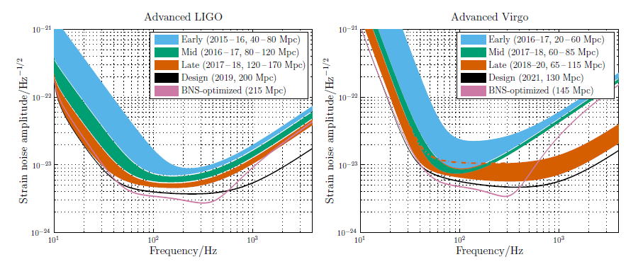
The anticipated strain sensitivity evolution for aLIGO and AdV is shown in Figure 1*. A standard figure of merit for the sensitivity of an interferometer is the BNS range : the volume- and orientation-averaged distance at which a compact binary coalescence consisting of two neutron stars gives a matched filter signal-to-noise ratio (SNR) of 8 in a single detector [58].¹ The BNS ranges for the various stages of aLIGO and AdV expected evolution are also provided in Figure 1*.

Figure 1: aLIGO (left) and AdV (right) target strain sensitivity as a function of frequency. The binary neutron-star (BNS) range, the average distance to which these signals could be detected, is given in megaparsec. Current notions of the progression of sensitivity are given for early, mid and late commissioning phases, as well as the final design sensitivity target and the BNS-optimized sensitivity. While both dates and sensitivity curves are subject to change, the overall progression represents our best current estimates.

The commissioning of aLIGO is well under way. The original plan called for three identical 4-km interferometers, two at Hanford (H1 and H2) and one at Livingston (L1). In 2011, the LIGO Lab and IndIGO consortium in India proposed installing one of the aLIGO Hanford detectors (H2) at a new observatory in India (LIGO-India) [64]. As of early 2015, LIGO Laboratory has placed the H2 interferometer in long-term storage for possible use in India. Funding for the Indian portion of LIGO-India is in the final stages of consideration by the Indian government.

Advanced LIGO detectors began taking sensitive data in August 2015 in preparation for the first observing run. O1 formally began 18 September 2015 and ended 12 January 2016. It involved the H1 and L1 detectors; the detectors were not at full design sensitivity. We aimed for a BNS range of 40 – 80 Mpc for both instruments (see Figure 1*), and both instruments were running with a 60 – 80 Mpc range. Subsequent observing runs will have increasing duration and sensitivity. We aim for a BNS range of 80 – 170 Mpc over 2016 – 2018, with observing runs of several months. Assuming that no unexpected obstacles are encountered, the aLIGO detectors are expected to achieve a 200 Mpc BNS range circa 2019. After the first observing runs, circa 2020, it might be desirable to optimize the detector sensitivity for a specific class of astrophysical signals, such as BNSs. The BNS range may then become 215 Mpc. The sensitivity for each of these stages is shown in Figure 1*.

As a consequence of the planning for the installation of one of the LIGO detectors in India, the installation of the H2 detector has been deferred. This detector will be reconfigured to be identical to H1 and L1 and will be installed in India once the LIGO-India Observatory is complete. The final schedule will be adopted once final funding approvals are granted. If project approval comes soon, site development could start in 2016, with installation of the detector beginning in 2020. Following this scenario, the first observing runs could come circa 2022, and design sensitivity at the same level as the H1 and L1 detectors is anticipated for no earlier than 2024.

The time-line for the AdV interferometer (V1) [23] is still being defined, but it is anticipated that in 2016 AdV will join the aLIGO detectors in their second observing run (O2). Following an early step with sensitivity corresponding to a BNS range of 20 – 60 Mpc, commissioning is expected to bring AdV to a 60 – 85 Mpc in 2017 – 2018. A configuration upgrade at this point will allow the range to increase to approximately 65 – 115 Mpc in 2018 – 2020. The final design sensitivity, with a BNS range of 130 Mpc, is anticipated circa 2021. The corresponding BNS-optimized range would be 145 Mpc. The sensitivity curves for the various AdV configurations are shown in Figure 1*.

The GEO 600 [76] detector will likely be operational in the early to middle phase of the AdV and aLIGO observing runs, i.e. 2015 – 2017. The sensitivity that potentially can be achieved by GEO in this time-frame is similar to the AdV sensitivity of the early and mid scenarios at frequencies around 1 kHz and above. GEO could therefore contribute to the detection and localization of high-frequency transients in this period. However, in the  100 Hz region most important for BNS signals, GEO will be at least 10 times less sensitive than the early AdV and aLIGO detectors, and will not contribute significantly.

Japan has begun the construction of an advanced detector, KAGRA [100, 28]. KAGRA is designed to have a BNS range comparable to AdV at final sensitivity. We do not consider KAGRA in this article, but the addition of KAGRA to the worldwide GW-detector network will improve both sky coverage and localization capabilities beyond those envisioned here [96*].

Finally, further upgrades to the LIGO and Virgo detectors, within their existing facilities (e.g., [63, 78, 11]) as well as future underground detectors (for example, the Einstein Telescope [93]) are envisioned in the future. These affect both the rates of observed signals as well as the localizations of these events, but this lies beyond the scope of this paper.

2.2 Envisioned observing schedule

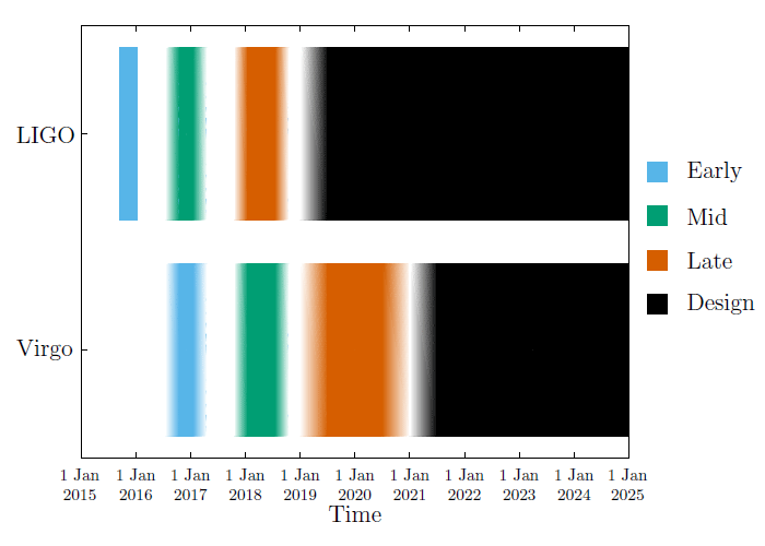
Keeping in mind the important caveats about commissioning affecting the scheduling and length of observing runs, the following is a plausible scenario for the operation of the LIGO–Virgo network over the next decade:

2015 – 2016 (O1)

A four-month run (beginning 18 September 2015 and ending 12 January 2016) with the two-detector H1L1 network at early aLIGO sensitivity (40 – 80 Mpc BNS range).

2016 – 2017 (O2)

A six-month run with H1L1 at 80 – 120 Mpc and V1 at 20 – 60 Mpc.

2017 – 2018 (O3)

A nine-month run with H1L1 at 120 – 170 Mpc and V1 at 60 – 85 Mpc.

2019+

Three-detector network with H1L1 at full sensitivity of 200 Mpc and V1 at 65 – 115 Mpc.

2022+

H1L1V1 network at full sensitivity (aLIGO at 200 Mpc, AdV at 130 Mpc), with other detectors potentially joining the network. Including a fourth detector improves sky localization [72, 109*, 79*, 91*], so as an illustration we consider adding LIGO-India to the network. 2022 is the earliest time we imagine LIGO-India could be operational, and it would take several more years for it to achieve full sensitivity.

This time-line is summarized in Figure 2*. The observational implications of this scenario are discussed in Section 4.

Figure 2: The planned sensitivity evolution and observing runs of the aLIGO and AdV detectors over the coming years. The colored bars show the observing runs, with the expected sensitivities given by the data in Figure 1*. There is significant uncertainty in the start and end times of the observing runs, especially for those further in the future, and these could move forward or backwards by a few months relative to what is shown above. The plan is summarised in Section 2.2.