Cosmological redshift-space distortion

5.3 Cosmological redshift-space distortion

Consider a spherical object at high redshift. If the wrong cosmology is assumed in interpreting the distance-redshift relation along the line of sight and in the transverse direction, the sphere will appear distorted. Alcock and Paczynski [2 ] pointed out that this curvature effect could be used to estimate the cosmological constant. Matsubara and Suto [54 ] and Ballinger, Peacock, and Heavens [3

] developed a theoretical framework to describe the geometrical distortion effect (cosmological redshift distortion) in the two-point correlation function and the power spectrum of distant objects, respectively. Certain studies were less optimistic than others about the possibility of measuring this Alcock–Paczynski effect. For example, Ballinger, Peacock, and Heavens [3 ] argued that the geometrical distortion could be confused with the dynamical redshift distortions caused by peculiar velocities and characterized by the linear theory parameter $0.6 β ≡ Ω m ∕b$ . Matsubara and Szalay [55 , 56 ] showed that the typical SDSS and 2dF samples of normal galaxies at low redshift ( $z ∼ 0.1$ ) have sufficiently low signal-to-noise, but they are too shallow to detect the Alcock–Paczynski effect. On the other hand, the quasar SDSS and 2dFGRS surveys are at a useful redshift, but they are too sparse. A more promising sample is the SDSS Luminous Red Galaxies survey (out to redshift $z ∼ 0.5$ ) which turns out to be optimal in terms of both depth and density.

While this analysis is promising, it remains to be tested if non-linear clustering and complicated biasing (which is quite plausible for red galaxies) would not ‘contaminate’ the measurement of the equation of state. Even if the Alcock–Paczynski test turns out to be less accurate than other cosmological tests (e.g., CMB and SN Ia), the effect itself is an interesting and important ingredient in analyzing the clustering pattern of galaxies at high redshifts. We shall now present the formalism for this effect.

Due to a general-relativistic effect through the geometry of the Universe, the observable separations perpendicular and parallel to the line-of-sight direction, $xs⊥ = (c∕H0 )zδ𝜃$ and $xs∥ = (c∕H0)δz$ , are mapped differently to the corresponding comoving separations in real space $x⊥$ and $x∥$ :

with $dA (z)$ being the angular diameter distance. The difference between $c⊥(z )$ and $c∥(z )$ generates an apparent anisotropy in the clustering statistics, which should be isotropic in the comoving space. Then the power spectrum in cosmological redshift space $P (CRD)$ is related to $P (S)$ defined in the comoving redshift space as

where the first factor comes from the Jacobian of the volume element $2 dks⊥dks∥$ , and $ks⊥ = c⊥(z)k⊥$ and $ks∥ = c∥(z)k∥$ are the wavenumber perpendicular and parallel to the line-of-sight direction.

Using Equation (131 ), Equation (156 ) reduces to

2 ( ∘ ----[---------]---- ) (CRD ) ---b-(z-)--- (R) --ks-- --1-- 2 P (ks,μk;z ) = c⊥(z)2c∥(z )Pmass c⊥(z) 1 + η(z)2 − 1 μk;z × ( ) [ ( 1 ) ]−2 [ ( 1 + β(z) ) ]2 k2μ2σ2 −1 1 + ----2 − 1 μ2k 1 + -----2---− 1 μ2k 1 + -s2k-P- , (157 ) η (z ) η(z) 2c∥(z)

where

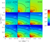
Figure 16 shows anisotropic power spectra $P (CRD)(ks,μk;z = 2.2)$ . As specific examples, we consider SCDM, LCDM, and OCDM models, which have $(Ω ,Ω ,h,σ ) = (1.0,0.0,0.5,0.6) m Λ 8$ , $(0.3,0.7,0.7,1.0 )$ , and $(0.3,0.0,0.7,1.0)$ , respectively. Clearly the linear theory predictions ( $σP = 0$ ; top panels) are quite different from the results of $N$ -body simulations (bottom panels), indicating the importance of the nonlinear velocity effects ( $σP$ computed according to [58 ]; middle panels).

Figure 16: Two-dimensional power spectra in cosmological redshift space at $z = 2.2$ . (Figure taken from [46

].)

Next we decompose the power spectrum into harmonics,

where $Ll(μk)$ are the $l$ -th order Legendre polynomials. Similarly, the two-point correlation function is decomposed as

using the direction cosine $μ x$ between the separation vector and the line-of-sight. The above multipole moments satisfy the following relations:

∫ --1-- ∞ 2 ξl(x;z ) = 2π2il Pl(k; z)jl(kx )k dk, (161 ) ∫ 0∞ P (k;z ) = 4πil ξ (x;z)j(kx )x2dx, (162 ) l 0 l l

with $jl(kx)$ being spherical Bessel functions. Substituting 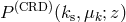$(CRD) P (ks,μk;z)$ in Equation (159

) yields $(CRD) P l (ks;z)$ , and then $ξ(CRD)(xs;z)$ can be computed from Equation (161

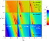
Figure 17: The confidence contours on the $Ωm$ - $Ω Λ$ plane from the $2 χ$ -analysis of the monopole and quadrupole moments of the power spectrum in the cosmological redshift space at $z = 2.2$ . We randomly selected $N = 5 × 103$ (upper panels), $N = 5 × 104$ (middle panels), and $N = 5 × 105$ (lower panels) particles from $N$ -body simulation. The value of $σ 8$ is adopted from the cluster abundance. (Figure taken from [46 ].)

A comparison of the monopoles and quadrupoles from simulations and model predictions exhibits how the results are sensitive to the cosmological parameters, which in turn may put potentially useful constraints on $(Ωm, ΩΛ)$ . Figure 17 indicates the feasibility, which interestingly results in a constraint fairly orthogonal to that from the supernovae Ia Hubble diagram.